

Binary Logistic Regression

“‘At its most fundamental, information is a binary choice. In other words, a single bit of information is one yes-or-no choice.’”
Objectives:
This blog focuses solely on binary logistic regression. Multinomial logit, discrete choice analysis, ordered data analysis, four-way data analysis, etc. will be published in subsequent blog posts. The below is a fairly robust discussion of all things binary logistic regression in the context of data science with Python.
Explore problems with dichotomous dependent variables;
Discuss odds and odds ratios;
Get introduced to the logistic regression model;
Gain an understanding of the general principles of estimation with logit models;
Discuss the maximum likelihood estimation method;
Understand convergence issues;
Assess the impact of multicollinearity;
Look at goodness-of-fit and predictive power; and
Get familiar with ROC curves and Precision-Recall curves.
A foreword of sorts:
Classification problems are the focus of many machine learning algorithms today. Classification predictions can be made with several methodologies, but the focus of this blog is logistic regression or logit analysis. More specifically, this blog entry explores logistic regression analysis of dichotomous dependent variables.
Dichotomous obviously means yes or no, and is often coded 1, if a condition exists, and 0 if it doesn’t. For example, a longitudinal study may follow people over a specified time period with the goal of finding out whether individuals developed a condition or not (e.g. developed diabetes or did not develop diabetes).
Can we use OLS Regression to solve a problem with a binary outcome?
We recall that there are five assumptions that must be satisfied for OLS regression to provide an unbiased estimate:
The dependent variable is a linear function of the independent variable(s) for all observations;
The error and independent variables are not correlated;
Homoscedasticity, e.g. the variance of error is the same for all observations of the independent variables;
Multicolliniarity, e.g. the error associated with one independent variable is not correlated wit the error associated with another independent variable; and
The error, or random disturbance, is normally distributed.
In binary logistic regression analysis (e.g. the dependent variable is binary), it is not possible to satisfy the homoscedasticity assumption and the assumed normal distribution of the error term. The other three requirements are still valid, however.
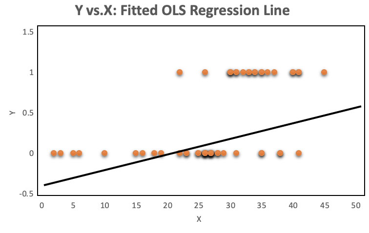
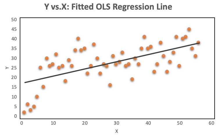
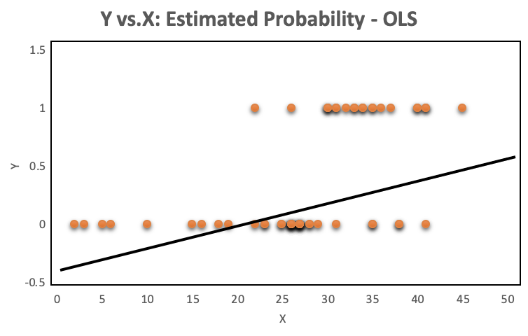
OLS Regression vs. Logit Model:
A look at the distribution of the data makes it even more obvious, why OLS regression should not be used for models where the dependent variable is dichotomous. The OLS regression line provides predictions above and below the bounded region of the observations, as shown on the left. The right chart with a continuous dependent variable has no such issue because the observations are not bounded to 0 and 1.
Odds and Odds Ratios:
The issue of bounding can be resolved by introducing odds as a dependent variable. More on that in a few minutes….
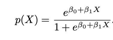
Before discussing how logistic regression works, a discussion about odds and odds ratios is warranted. The relationship between probabilities and odds can be written as
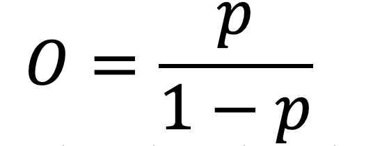
which is the probability of an even divided by the probability of no event. With the formula above, it is easy to create the following table.

Odds make more sense for modeling. For example, if the probability of an event taking place is 70%, it is not possible to express the probability of an even that is twice that. We have no such issue with odds. The odds when the probability is 70% are 2.33, therefore twice that is 4.66. This can be converted back to probability if needed using the same formula…
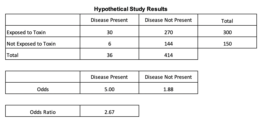
The data for the hypothetical study below was sourced from NCBI (Click for article). Odds can be used to compute odds ratios, which are especially useful when using binary variables. The odds ratio in the below table is the quotient of the odds of the presence of the disease for those exposed vs. not exposed to a toxin. The odds of having the disease after being exposed to a toxin in this example is 167% higher than the odds of having the disease when not being exposed to the toxin. Since odds ratios are less prone to be affected by extreme values , the construct is frequently used in scientific literature when describing relationships of two variables.
From the table, it is obvious that odds that are associated with probabilities lower than 0.5 are less than one and the value of odds corresponding to probabilities greater than 0.5 are higher than one.
So to make the point one more time: Since binary variables are bounded by 0 and 1 and linear functions are unbounded, the probabilities need to be transformed so that they too are unbounded. As described earlier, transforming probabilities to odds removes the issue of bounding.
The Logit Model:
Modeling the probability of an observation belonging to one of two classes with linear regression is inappropriate. James et al. (Introduction to Statistical Learning) provide an excellent explanation of the issue:
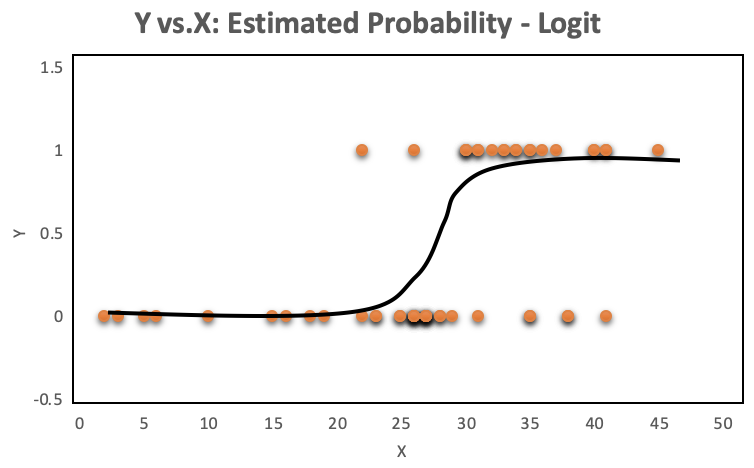
The orange plots indicate yes or no events. The left chart shows a fitted liner regression curve, while the right hand chart shows a logistic regression utilizing the sigmoid curve. Logistic regression performs better!
So logistic regression is more appropriate when the response is binary, and the equation to use is below. Note the sigmoid function, which generates the S shaped curve.
To fit a logistic model, maximum likelihood is a good approach. Maximum likelihood is a popular way to estimate the logit model because of its consistency and convenience. Some manipulation is needed, but it is possible to rearrange the probability equation above so that the left hand side contains odds, rather than probabilities, which can take any value between zero and infinity.

Taking the log of both sides gives us the equation that the model is named after, since the left side of the equation contains the log of odds or logit. Note that there is no error term. The logit equation can be solved for p and then further simplified . A single variable with alpha set to 0 and beta to 1will produce an S shaped curve. When X is either small or large it gets close to 0 or 1 but never equals those boundaries.

Binary Logistic Regression with Python:
The goal is to use machine learning to fit the best logit model with Python, therefore Sci-Kit Learn(sklearn) was utilized. A dataset of 8,009 observations was obtained from a charitable organization. The data contained 24 variables that provided information about potential donors’ demographic information, financials and previous donation/gifting behavior. Logistic regression was used to identify (predict) potential donors.
First, the necessary libraries need to be loaded:
import numpy as np
import pandas as pd
import seaborn as sns
import matplotlib.pyplot as plt
import seaborn as sns
import statsmodels.api as sm

import sklearn
from sklearn import metrics
from sklearn.metrics import roc_auc_score

from sklearn.model_selection import train_test_split
from sklearn.linear_model import LogisticRegression
from sklearn.metrics import classification_report
from sklearn.metrics import confusion_matrix

%matplotlib inline
Next, read the csv file and take a look at the first few rows and columns. The first obvious point is that the data has some missing values.
#read csv file
charity_df = pd.read_csv('charity.csv')
charity_df.head()

charity_df.isnull().sum()
#remove all lines with missing observations
charity_df=charity_df.dropna()
There were 2,007 observations with missing values, which were removed from analysis to make things simple. The data is now ready for EDA. Since the blog is focused on logistic regression, I deliberately kept the EDA section short. I simply wanted to show some of the steps that are useful but certainly others may me appropriate as well. I find the seaborn package very useful for preliminary visualization.
#Exploratory Data Analysis
#Bivariate plots
sns.jointplot('lgif', 'rgif', data=charity_df)
#Heatmap of correlations
sns.heatmap(charity_df.corr())

#Distributions
fig = plt.figure(figsize=(15, 12))

# loop over all vars (total: 24)
for i in range(1, charity_df.shape[1]):
    plt.subplot(6, 6, i)
    f = plt.gca()
    f.axes.get_yaxis().set_visible(False)
    # f.axes.set_ylim([0, train.shape[0]])
    vals = np.size(charity_df.iloc[:, i].unique())
    if vals < 10:
        bins = vals
    else:
        vals = 10
    plt.hist(charity_df.iloc[:, i], bins=30, color='#3F5D7D')
plt.tight_layout()
An Example of a Bivariate Plot with Distributions

An Example of a Heat Plot with Correlations

Histograms of All Variables

Partitioning the data creates a train and test dataset. Before partitioning, the variable damt was removed. That variable contains the amount donated in the past, and can be used for predictive modeling when the amount donated is predicted. In the current exercise case, we are not interested in that variable.
In the code below, you will notice that I also removed several other variables. This is due to a model I built earlier that suggested the removal of these variables. I wanted to make the current exercise a bit more streamlined, hence this step. We can see that the remaining data was split into 4,801 training and 1,201 test observations. I also listed the variables that remained, which we will place into the regression.
#Partition the data

#first drop damt
charity_df = charity_df.drop('damt', axis=1)
charity_df.head()

#Create training and test datasets

#Create regressors and dependent variable
#note that donr was dropped from X because it is the dependent variable
#all other variables dropped here were identified as not significant contributors to reg
X = charity_df.drop(['donr', 'reg3', 'reg4','hinc','genf','avhv', 'lgif', 'rgif', 'agif'], axis=1)
y = charity_df['donr']

print(list(X.columns.values))

X_train, X_test, y_train, y_test = sklearn.model_selection.train_test_split(X, y, test_size = 0.20, random_state = 5)
print(X_train.shape)
print(X_test.shape)
print(y_train.shape)
print(y_test.shape)

['ID', 'reg1', 'reg2', 'home', 'chld', 'wrat', 'incm', 'inca', 'plow', 'npro', 'tgif', 'tdon', 'tlag']
(4801, 13)
(1201, 13)
(4801,)
(1201,)
Sci-kit Learn offers LogisticRegression for the training of binary logit models. While I kept everything simple here, there are lots of options. For example, take a look at the coded out section in red. The detailed user guide can be found by clicking here.
Penalty allows the specification of penalty terms, such as l1, l2 or elasticnet. Note that some solver options require a specific penalty specified. In the solution below I selected none to match the solution when using the statsmodels package. This requires us to change the solver type, since the default is not compatible with no penalty.
Random_state helps reproducing the solution by specifying a seed,
Solver means the algorithm that is used in the optimization problem. This is an important area to read in the user guide because it may be the source of significant heartache. The some choices are in direct conflict with other tunable specifications of LinearRegression. Since I wanted to match the results of the statsmodels package, I changed the solver to newton-cg.
Multi_class is an option that allows us to specify whether we are fitting binary or multinomial logit models. The option ‘ovr’ is to be used for a binary dependent variable.
fit_intercept enables the use of an intercept. The default is True.
Other options are: tol, C, intercept_scaling, class_weight, max_iter, verbose, warm_start, n_jobs, 1_ratio
model1 = LogisticRegression(random_state=0, multi_class='ovr', penalty='none', solver='newton-cg').fit(X_train, y_train)
The object preds stores the predicted y values of the model when the model is deployed on the test data. This will be used extensively to judge the model.
Here are the actual parameters used in the model. Note the changes made from default for penalty and the solver.
preds = model1.predict(X_test)
params = model1.get_params()
params

{'C': 1.0,
 'class_weight': None,
 'dual': False,
 'fit_intercept': True,
 'intercept_scaling': 1,
 'l1_ratio': None,
 'max_iter': 100,
 'multi_class': 'ovr',
 'n_jobs': None,
 'penalty': 'none',
 'random_state': 0,
 'solver': 'newton-cg',
 'tol': 0.0001,
 'verbose': 0,
 'warm_start': False}
We can now print the intercept and the parameter estimates:
#Print model parameters
print('Intercept: \n', model1.intercept_)
print('Coefficients: \n', model1.coef_)

Intercept:
 [-4.1233617]
Coefficients:
 [[ 1.26524129e+00  2.40687467e+00  3.44423683e+00 -1.35081254e+00
   3.31638202e-01  1.46360352e-02 -1.15610992e-03 -1.37226498e-02
   1.20037090e-02  1.59873872e-03 -5.16934518e-02 -1.26923128e-01]]
The above model is reproducible with the statsmodels package, which provides a very convenient way of obtaining goodness-of-fit statistics. Fit statistics are stored in summary() and in summary2(). As always, we must not forget to add a constant for the y-intercept.
#Use statsmodels to assess fit

logit_model=sm.Logit(y_train,sm.add_constant(X_train))
logit_model
result=logit_model.fit()
stats1=result.summary()
stats2=result.summary2()
print(stats1)
print(stats2)
The first table shows the models’ degrees of freedom and the pseudo R-squared. Pseudo R-squared is similar to the R-squared statistic for OLS regression but it is computed based on the ratio of the maximized log-likelihood function for the null model m0 and the full model m1. For more from the statsmodels documentation click here.
The table also provides statistics about each of the features. The parameter estimates and their associated standard errors, z scores and significance stats are given along with confidence intervals. The second table provides AIC, and BIC values in addition to statistics about the features. This is very useful if one does not want to write additional code to compute the AIC and BIC.
AIC = -2logL + 2k where k is the number of parameters including the intercept
BIC = -2logL + klogn where n is the sample size
AIC and BIC are fit statistics that penalize models with more covariates. In fact, BIC penalizes even more severely for a higher number of covariates. Both fit statistics are meaningful to compare models with different sets of covariates.
LL-Null is the result of the maximized log-likelihood function when only an intercept is included, and the LLR p-value determines whether the specified model is better than having no features. Another way of asking this is whether all regression coefficients are zero. They clearly are not in this example.

Interpretation of Coefficients:
The table above lists all coefficients. One of them (inca) is not significant and should be removed. But how do we interpret these coefficients? For example, what does the 1.27 mean for reg1? Since these are logit coefficients, the reg1 coefficient means that for every one unit increase in reg1, there will be a 1.27 increase in the log-odds of the outcome variable, in this case becoming a donor. Since the logit model assumes a non-linear relationship between independent and dependent variables, the change in the probability of the outcome for a single unit increase in a regressor varies according to where the observation starts. However, we can calculate the odds ratio estimates by taking the exponent of each coefficient. These are adjusted ratios because they control for other variables in the model. The 3.54 odds ratio estimates that the predicted odds of becoming a donor is 254% higher if a person lives in reg1 vs. if he or she does not. Reg1 happens to be a dummy variable, but the interpretation will work the same way for other variables. This way, the interpretation of the coefficients makes more sense.
#Calculate odds ratio estimates
import numpy as np
np.exp(model1.coef_)

array([[ 3.54394774, 11.09921811, 31.31937247,  0.2590297 ,  1.39324868,
         1.01474367,  0.99884456,  0.98637108,  1.01207604,  1.00160002,
         0.94961993,  0.88080138]])
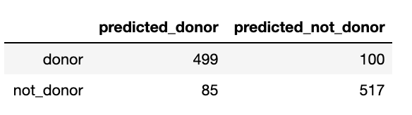
Confusion Matrix:
The command confusion_matrix creates an array, that shows the number of true positives (TP), false positives (FP), false negatives (FN) and true negatives (TN). These figures will be used extensively for the assessment of the model. But first, let us take a look at what the confusion matrix actually looks like in a 2 by 2 table.
#Create a confusion matrix
#y_test as first argument and the preds as second argument
confusion_matrix(y_test, preds)

array([[499, 100],
       [ 85, 517]])
#transform confusion matrix into array
#the matrix is stored in a variable called confmtrx
confmtrx = np.array(confusion_matrix(y_test, preds))

#Create DataFrame from confmtrx array
#rows for test: donor or not_donor designation as index
#columns for preds: predicted_donor or predicted_not_donor as column

pd.DataFrame(confmtrx, index=['donor', 'not_donor'],
columns=['predicted_donor', 'predicted_not_donor'])
With the data in hand, we can calculate several important statistics to assess the accuracy of our model. Some of what is calculated below is also available in the summary report, but some of the nomenclature is not as intuitive.
confusion = pd.DataFrame(confmtrx, index=['donor', 'not_donor'],
columns=['predicted_donor', 'predicted_not_donor'])

TP = confusion.ix['donor', 'predicted_donor']
FP = confusion.ix['not_donor', 'predicted_donor']
TN = confusion.ix['not_donor', 'predicted_not_donor']
FN = confusion.ix['donor', 'predicted_not_donor']

#Reproduce classifcation report
TPR=(float(TP) / (TP + FN))
TPN=(float(TN) / (TN + FP))
PPV=(float(TP) / (TP + FP))
NPV=(float(TN) / (TN + FN))
FNR=(float(FN) / (FN + TP))
FPR=(float(FP) / (FP + TN))
FDR=(float(FP) / (FP + TP))
FOR=(float(FN) / (FN + TN))
TS=(float(TP) / (TP+FN + FP))
ACC=(float(TP+TN) / (TP+FP+FN + TN))  #print((TP + TN) / float(len(y_test)))
F1=2*TP/(2*TP+FP+FN)

print ("sensitivity, recall, hit rate, or true positive rate (TPR): ",TPR)
print ("specificity, selectivity or true negative rate (TNR): ",TPN)
print ("precision or positive predictive value (PPV): ",PPV)
print ("negative predictive value (NPV): ",NPV)
print ("miss rate or false negative rate (FNR): ",FNR)
print ("fall-out or false positive rate (FPR): ",FPR)
print ("false discovery rate (FDR): ",FDR)
print ("false omission rate (FOR): ",FOR)
print ("Threat score (TS) or Critical Success Index (CSI): ",TS)
print("")
print ("accuracy (ACC): ",ACC)
print ("F1: ",F1)

sensitivity, recall, hit rate, or true positive rate (TPR):  0.8330550918196995
specificity, selectivity or true negative rate (TNR):  0.8588039867109635
precision or positive predictive value (PPV):  0.8544520547945206
negative predictive value (NPV):  0.8379254457050244
miss rate or false negative rate (FNR):  0.1669449081803005
fall-out or false positive rate (FPR):  0.14119601328903655
false discovery rate (FDR):  0.14554794520547945
false omission rate (FOR):  0.1620745542949757
Threat score (TS) or Critical Success Index (CSI):  0.72953216374269

accuracy (ACC):  0.8459616985845129
F1:  0.8436179205409975
Several statistics about the accuracy of the model are available in sklearn.metrics as specific objects. We can obtain a classification report as well (or instead of the individual items above), which contains all important metrics.
#Accuracy statistics
import sklearn
from sklearn import metrics

print('Accuracy Score:', metrics.accuracy_score(y_test, preds))
print('Average Precision Score:', metrics.average_precision_score(y_test, preds))
print('F1 Score:', metrics.f1_score(y_test, preds))
print('Precision:', metrics.precision_score(y_test, preds))
print('Recall:', metrics.recall_score(y_test, preds))

#Create classification report
class_report=classification_report(y_test, preds)
print(class_report)

Accuracy Score: 0.8459616985845129
Average Precision Score: 0.7903880680424489
F1 Score: 0.8482362592288762
Precision: 0.8379254457050244
Recall: 0.8588039867109635
              precision    recall  f1-score   support

         0.0       0.85      0.83      0.84       599
         1.0       0.84      0.86      0.85       602

    accuracy                           0.85      1201
   macro avg       0.85      0.85      0.85      1201
weighted avg       0.85      0.85      0.85      1201
ROC Curve:
ROC stands for Receiver Operating Characteristic, which is a World War II term used to evaluate the performance of radar. We discussed specificity and sensitivity before, but to refresh: sensitivity is the proportion of correctly predicted events (cases), while specificity is the the proportion of correctly identified non-events (cases). Ideally, both specificity and sensitivity should be high. The ROC curve represents the tradeoff between the two constructs. The 45-degree blue line represents a model with an intercept and no variables, e.g. a model with no predictive value. Larger deviation from the 45-degree line means more predictive power. The graphs shows the area under the curve (0.93), which one would prefer to be as close to one as possible.
#Draw ROC Curve
y_pred_proba = model1.predict_proba(X_test)[::,1]
fpr, tpr, _ = metrics.roc_curve(y_test,  y_pred_proba)
roc_auc = metrics.roc_auc_score(y_test, y_pred_proba)
plt.plot(fpr,tpr,label="ROC Curve area="+str(roc_auc), color='darkorange')
plt.plot([0, 1], [0, 1], color='navy', linestyle='--')
plt.xlabel('False Positive Rate (1-Specificity)')
plt.ylabel('True Positive Rate (Sensitivity)')
plt.title('ROC Curve: Donor Model')
plt.legend(loc="lower right")

plt.show()

Precision-Recall Curve:
Precision and recall were described earlier in this blog, but to restate:
Precision (or positive predictive value): True positive / (True positive + False positive)
Recall (or sensitivity): True positive / (True positive + False negative)
One would prefer both precision and recall to be as high as possible, but similar to the ROC curve, the two need to be simultaneously maximized, which is difficult.
Precision and recall are especially important when the observations of the outcome are poorly balanced, and there are very few of positive or negative outcomes. If there are a large number of negative outcomes but only a few positive outcomes, then a model may be very accurate, but perform poorly when it comes to the prediction of positive outcomes.
The precision-recall curve contains a flat blue line representing a model with no predictive value. When the data is balanced, the line is at 0.5. This is the case for the current example as approximately 50% of all observations in the data were donors. We are looking for a point on the chart that represents a good mix of precision and recall. We can then assess the accuracy of the model at that point, to judge whether a model is acceptable or not.
#Draw precision-recall curve
from sklearn.metrics import precision_recall_curve

y_pred_proba = model1.predict_proba(X_test)[::,1]
precision, recall, _ = precision_recall_curve(y_test, y_pred_proba)
f1=metrics.f1_score(y_test, preds)
auc=metrics.roc_auc_score(y_test, preds)
plt.plot([0, 1], [0.5, 0.5], color='navy', linestyle='--', label='No Pred. Value')
plt.plot(recall, precision, label='logit', color='darkorange')
plt.xlabel('Recall')
plt.ylabel('Precision')
plt.title('Precision-Recall Curve: Donor Model')
plt.legend(loc="upper right")
plt.show()

Multicollinearity:
Logistic regression and OLS regression share several attributes. One of those is multicollinearity, as both methods are highly affected by variables that are correlated with each other. Multicollinearity makes variables unstable with large standard errors. Some variables end up having an overstated effect as a result of being in a correlated group. You can find a discussion about how to detect and treat multicollinearity in one of my prior blogs.
Based on the VIF scores below, the current model does not appear to suffer from multicollinearity.
#Multicollinearity
import statsmodels.api as sm
from statsmodels.stats.outliers_influence import variance_inflation_factor

# For each X, calculate VIF and save in dataframe
x_temp = sm.add_constant(X_train)

vif = pd.DataFrame()
vif["VIF Factor"] = [variance_inflation_factor(x_temp.values, i) for i in range(x_temp.values.shape[1])]
vif["features"] = x_temp.columns
print(vif.round(1))

  VIF Factor features
0         55.5    const
1          1.2     reg1
2          1.2     reg2
3          1.0     home
4          1.0     chld
5          1.0     wrat
6          4.4     incm
7          4.2     inca
8          1.8     plow
9          2.2     npro
10         2.2     tgif
11         1.0     tdon
12         1.0     tlag
