

Principal Components Analysis

““To tell you the truth, I’ve never met anybody who can envision more than three dimensions. There are some who claim they can, and maybe they can; it’s hard to say.””
Principal Components Analysis:
Principal Components Analysis (PCA) may mean slightly different things depending on whether we operate within the realm of statistics, linear algebra or numerical linear algebra. In statistics, PCA is the transformation of a set of correlated random variables to a set of uncorrelated random variables. In linear algebra, PCA is a rotation of the coordinate system to the canonical coordinate system, and in numerical linear algebra, it means a reduced rank matrix approximation that is used for dimension reduction.
Principal Component Analysis is the process of computing principal components and use those components in understanding data. (Source: James, et al.)
Uses for PCA:
PCA is used in two broad areas: a.) as a remedy for multicollinearity and b.) as a dimension reduction tool. In either case, we seek to understand the covariance structure in multivariate data.
In dimension reduction, which requires us to create a reduced rank approximation to the covariance structure, PCA can be used to approximate the variation in p prediction variables using k<p principal components. In other words, in PCA, a large set of correlated variables can be summarized with a smaller number of variables that explain most of the variability in data.
PCA can also be used to create a set of orthogonal variables from a set of raw predictor variables, which is a remedy for multicollinearity, and a precondition to cluster analysis.
Principal Components:
In a dataset of p features we could create bivariate scatter plots of all variable pairs to understand our data. In a large dataset with many features, this is not practical, and it is possible that most pairs of features would contribute very little to our understanding of the data. PCA helps us to create a two-dimensional plot of the data that captures most of the information in a low-dimensional space. A small number of dimensions are created to maximize data understanding based on observations’ variability along each dimension.
Finding Principal Components:
The first principal component of a set of variables is the standardized linear combination of the original variables with the largest variance among all linear combinations. The second principal component is the standardized linear combination of original variables with the largest variance among all remaining linear combinations, given that the second principal component is not correlated with the first principal component. The third, fourth…nth principal components are defined in a similar way.
In reality, it means that we compute the eigenvalue-eigenvector pairs using a matrix factorization called Singular Value Decomposition (SVD).

Assumptions:
PCA does not require statistical assumptions. However, it is sensitive to the scale of the data. As a result, the data must be standardized (standard deviation = 1 and mean =0). This means that column means in the n*p matrix will be 0. The PCA of the data needs to be based on the correlation matrix, not on the covariance matrix. Note that the principal components predict the observed covariance matrix.
Selection of the Number of Factors to Retain:
There are three widely used methods to selecting the number of factors to retain: a.) scree plot, b.) Kaiser rule, c.) percent of variation threshold. It is always important to be parsimonious, e.g. select the smallest number of principal components that provide a good description of the data.
A visual approach to selecting the number of principal components to keep means the use of a scree plot. A scree plot shows the number of components on the X-axis against the proportion of the variance explained on the Y-axis. The suggested number of components to keep is where the plot forms an elbow and the curve flattens out. Unfortunately, the scree plot often presents some ambiguity. Further, a practical approach often prompts analysts to evaluate the first few principal components, and if they are of interest, the analyst would continue considering additional principal components. However, if the first few principal components provide little relevance, evaluation of additional principal components is likely of no use.
The Kaiser rule suggests the minimum eigenvalue rule. In this case, the number of principal components to keep equals the number of eigenvalues greater than 1.
Finally, the number of components to keep could be determined by a minimal threshold that explains variation in the data. In this case, we would keep as many principal components as needed to explain at least 70% (or some other threshold) of the total variation in the data.
The Pythonian Solution to PCA:
In this example, we will be working with baseball data! The dataset contains statistics about each major league baseball team’s performance between 1871 and 2006. There are 16 variables and about 2,200 records to play with. We will try to reduce the number of features to get a more manageable set.

I quickly created an additional variable by quantiling the number of wins. In fact, I generated three equal groups based on the sorted number of wins (TARGET_WINS). I selected the best third and called the quantile 1st 33%. I also created second and third groups and called them 2nd 33% and 3rd 33% respectively. This is just so that I can create interesting plots later in the analysis. (Plus its good to see how to quickly quantile data.)
baseball_df=baseball_df.sort_values('TARGET_WINS')
baseball_df['WINS_GROUP']=pd.qcut(baseball_df['TARGET_WINS'], 3, labels=['1st 33%','2nd 33%','3rd 33%'])
After ingesting the data, I found that there were a lot of missing observations. One feature was particularly poor in data capture (TEAM_BATTING_HBP), so I simply dropped it. I also filled missing values with the column means.
final_df=baseball_df.drop(['TEAM_BATTING_HBP', 'INDEX', 'WINS_GROUP'], axis=1)
final_df=final_df.fillna(final_df.mean())
We discussed the importance of standardizing, and here I used the StandardScaler() option to ensure that all features have a standard deviation of 1 and a mean of 0. We are ready for principal component analysis.
scaler = StandardScaler()

scaled_baseball=final_df.copy()
scaled_baseball=pd.DataFrame(scaler.fit_transform(scaled_baseball), columns=scaled_baseball.columns)
scaled_baseball.head()

In this example, I specified to create six principle components using Sci-kit Learn’s decomposition.PCA library . The svd solver was set to auto (the default). It is possible to use alternate specifications for the svd solver: auto, full, arpack, and randomized. Some of these settings allow concurrent modification of other parameters.
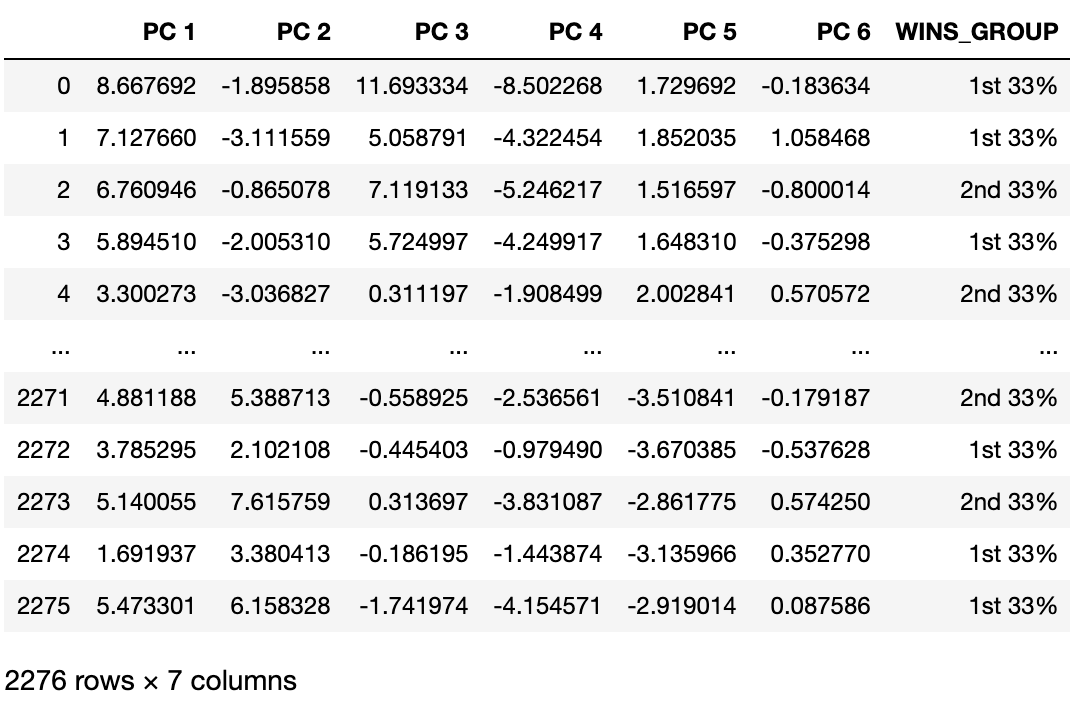
Here we can see the six principal components and the 2,276 observations.
pca = PCA(n_components=6, svd_solver == 'auto') Principal_components=pca.fit_transform(scaled_baseball) pca_df = pd.DataFrame(data = Principal_components, columns = ['PC 1', 'PC 2', 'PC 3', 'PC 4', 'PC 5', 'PC 6']) print(pca_df) PC 1 PC 2 PC 3 PC 4 PC 5 PC 6 0 8.667692 -1.895858 11.693334 -8.502268 1.729692 -0.183634 1 7.127660 -3.111559 5.058791 -4.322454 1.852035 1.058468 2 6.760946 -0.865078 7.119133 -5.246217 1.516597 -0.800014 3 5.894510 -2.005310 5.724997 -4.249917 1.648310 -0.375298 4 3.300273 -3.036827 0.311197 -1.908499 2.002841 0.570572 2271 4.881188 5.388713 -0.558925 -2.536561 -3.510841 -0.179187 2272 3.785295 2.102108 -0.445403 -0.979490 -3.670385 -0.537628 2273 5.140055 7.615759 0.313697 -3.831087 -2.861775 0.574250 2274 1.691937 3.380413 -0.186195 -1.443874 -3.135966 0.352770 2275 5.473301 6.158328 -1.741974 -4.154571 -2.919014 0.087586
For visualization, let us concatenate the observations with the each observations designation in terms of wins in a season. Remember, we quantiled each season by team into the top, middle and bottom 33% of the approximately 2,200 observations.
for_visual = pd.concat([pca_df, baseball_df['WINS_GROUP']], axis = 1)
print(for_visual)
We can create bivariate plots of each principal component against each principle component. In this example, I simply plotted the first two principle components, which is analogous to printing the original data to a low-dimensional subspace. Some of these are more interesting in real life than the one plotted here.
fig = plt.figure(figsize = (8,8))
ax = fig.add_subplot(1,1,1)
ax.set_xlabel('PC 1', fontsize = 15)
ax.set_ylabel('PC 2', fontsize = 15)
ax.set_title('Plot of 1st Two Principal Components vs. Wins', fontsize = 20)
W_GROUP = ['1st 33%','2nd 33%','3rd 33%']
colors = ['navy', 'turquoise', 'darkorange']
for WINS_GROUP, color in zip(W_GROUP,colors):
    indicesToKeep = for_visual['WINS_GROUP'] == WINS_GROUP
    ax.scatter(for_visual.loc[indicesToKeep, 'PC 1']
               , for_visual.loc[indicesToKeep, 'PC 2']
               , c = color
               , s = 50)
ax.legend(W_GROUP)
ax.grid()

Selecting the Number of Principal Components:
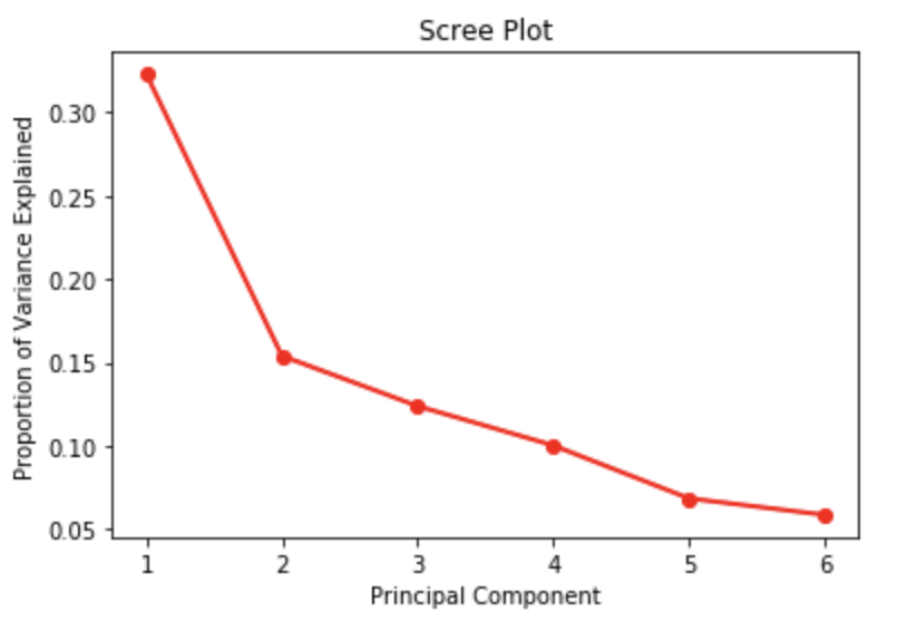
We have principle components, but how do we determine how many to keep. Let us work through the three approaches discussed earlier. The first is the scree plot solution. As discussed earlier, the scree plot is not completely transparent. Here we can observe an elbow at 2 and at 5 principle components. It seems that giving up the last principal component will not cost us much in terms of the explanatory power of our PCA.
import numpy as np
import matplotlib
import matplotlib.pyplot as plt

PC_values = np.arange(pca.n_components_) + 1
plt.plot(PC_values, pca.explained_variance_ratio_, 'ro-', linewidth=2)
plt.title('Scree Plot')
plt.xlabel('Principal Component')
plt.ylabel('Proportion of Variance Explained')
plt.show()
Next, let us try the threshold of variance explained approach. In this case, we hold on to principal components that explain at least 70% of the variance cumulatively. With the fourth principal component, the cumulative proportion of the variance explained surpasses 70%, therefore we would consider to keep four principal components. If a higher threshold were used, then additional principal components would have to be retained.
print ("Proportion of Variance Explained : ", pca.explained_variance_ratio_)

out_sum = np.cumsum(pca.explained_variance_ratio_)
print ("Cumulative Prop. Variance Explained: ", out_sum)

Proportion of Variance Explained :  [0.32272604 0.15399155 0.12394602 0.10037712 0.06864445 0.05877295]
Cumulative Prop. Variance Explained:  [0.32272604 0.47671759 0.60066362 0.70104074 0.76968519 0.82845815]
Finally, we could consider to hold onto principal components whose eigenvalues are greater than one. The eigenvalues are sum of squares of the distance between the projected data points and the origin along an eigenvector associated with a principal component. These are stored in the explained_variance attribute. Interestingly, the first five eigenvalues are above one, therefore we would need to drop only the last principal component and hold onto five of them. Whichever approach we prefer, Sci-Kit Learn does a great job providing the tools to make decisions.
print(pca.explained_variance_)

[4.84301852 2.31088859 1.86000756 1.50631866 1.03011941 0.88198182]
Factor loadings:
As a final point, we need to interpret our final PCA solution. The first principal component has strong loadings from TEAM_BATTING_3B (0.337590) and TEAM_FIELDING_E (0.354983). These are triples by batters and errors. If you are a baseball fan, you’d be able to evaluate whether any of this makes sense, but at least, everyone should be able to interpret the table below.
loadings = pd.DataFrame(pca.components_.T, columns=['PC1', 'PC2', 'PC3', 'PC4', 'PC5', 'PC6'], index=final_df.columns)
loadings

