Ensemble Methods: Bagging and Random Forests

““Don’t keep looking for ‘something’ in the bag of ‘nothing’. You will see the same thing again and again no matter how many times you repeat the look.””

— Israelmore Ayivor

Objectives:

• Gain an understanding of bootstrapping;

• Learn how to use Sci-kit Learn to build ensemble learning models;

• Demonstrate the use of ensemble learning models for regression:

  • Bagging;

  • Random forests;

• Compare bagging and random forests.

Bagging:

The bootstrap approach can be used to dramatically improve the performance of decision trees. Decision trees often suffer from relatively high variance, which results in poor accuracy measured on the test data. Bootstrap aggregation or bagging means that repeated samples are taken from a single training dataset with replacement. Regression trees are separately fitted on each, and each model is used for predictions. These predictions are then averaged.

Bootstrap:

Bootstrapping can be used to quantify the uncertainty pertaining to machine learning algorithms. It relies on a process that generates new sample sets from a population to estimate variability. In other words, sample data sets are repeatedly taken from a larger data set with replacement The standard error of the bootstrap samples is computed, and the average of these standard errors are used to estimate the standard error of the population. Both figures below are from Elements of Statistical Learning.

Histogram on left: estimates of alpha obtained by generating 1,000 simulated datasets from a true population. Center: estimates of alpha obtained from 1,000 bootstrap samples from a single data set. In each set, the pink line represents the tru value of alpha. (Elements of Statistical Learning)

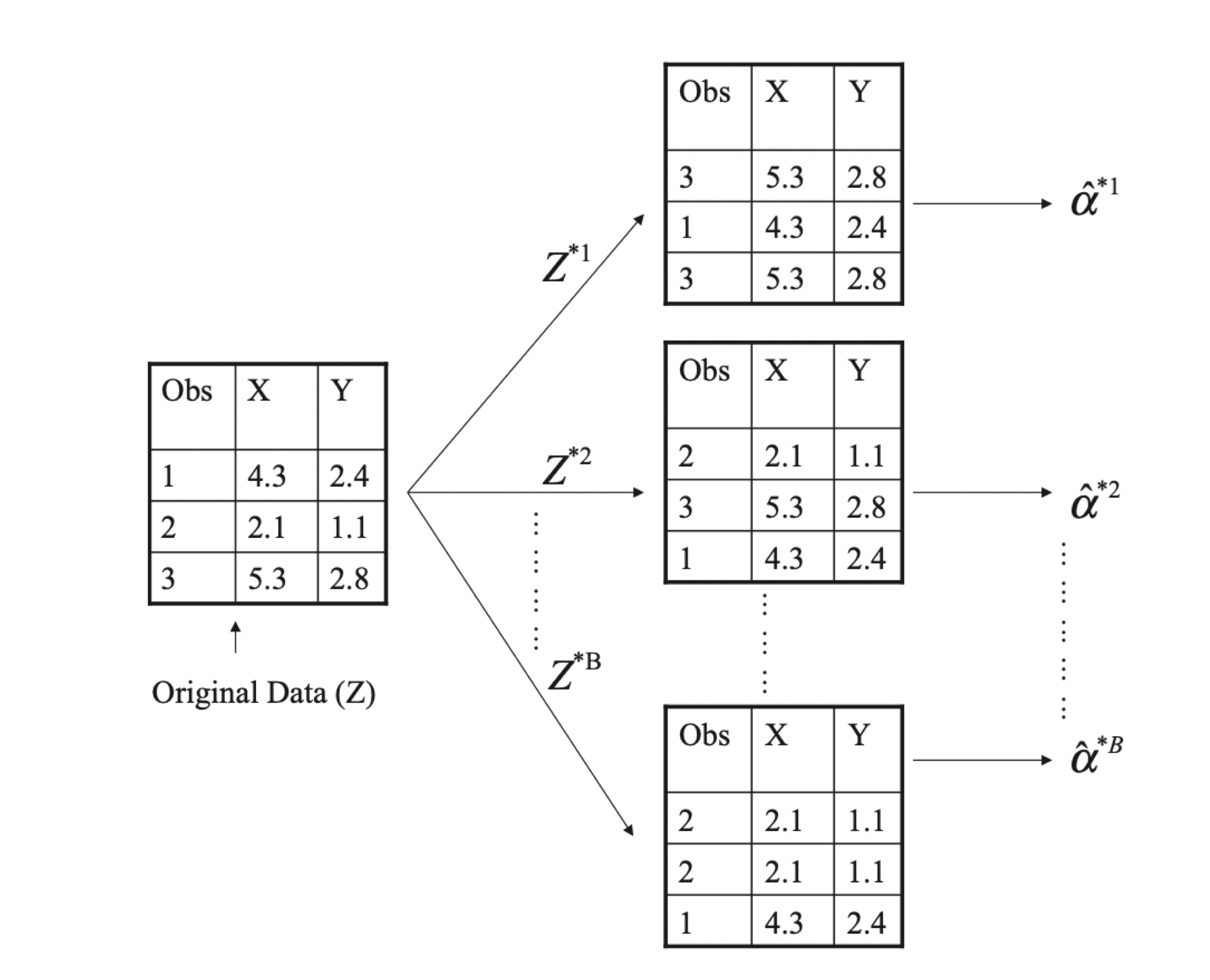
A visual representation of the bootstrap with three observations. Each bootstrap sample contains the same number of observations and are sampled with replacement. (Elements of Statistical Learning)

Ensemble Methods:

Bagging belongs to a group of statistical learning techniques called ensemble methods because multiple trees are being cultivated at the same time. However, unlike regression trees, the trees grown during bagging are not pruned, which means that they have high variance but low bias on an individual basis. Fortunately, the averaging of the predicted values significantly reduces variance for the system.

The test error is easy to compute. When fitting bagged trees, each uses approximately two-thirds of the of the observations, while one-third is not used and is often called out-of-bag observations. This can be used to compute OOB MSE for regression problems. It has been shown that OOB MSE is virtually the same as leave-one-out cross-validation error.

Challenges in Interpretation:

Unfortunately, the resulting model is cumbersome to interpret. When a lot of trees are used, it is impossible to tell the structure of decision making by the model. The importance of predictors is still possible to compute by understanding how much the RSS decreases on average at all splits for each individual predictor when building regression trees.

import numpy as np
import matplotlib.pyplot as plt
import pandas as pd  
import sklearn
from sklearn.ensemble import BaggingRegressor
from sklearn.tree import DecisionTreeRegressor
from sklearn.ensemble import RandomForestRegressor
from sklearn.model_selection import ParameterGrid
from sklearn import ensemble
from sklearn.metrics import mean_squared_error
from sklearn.utils import shuffle
from sklearn.datasets import load_boston

boston= load_boston()
boston_features_df = pd.DataFrame(data=boston.data,columns=boston.feature_names)
boston_target_df = pd.DataFrame(data=boston.target,columns=['MEDV'])

X_train, X_test, y_train, y_test = sklearn.model_selection.train_test_split(boston_features_df, boston_target_df, test_size = 0.20, random_state = 5)

#create arrays
#use ravel() for y_test and y_train to align with one dimensional array expectation
X_tra=X_train.values 
X_tes=X_test.values
y_tra=y_train.values.ravel()
y_tes=y_test.values.ravel()

At first, I created a parameter grid, which was then used for tuning during the bagging process. Special attention should be paid to the max_samples and max_features parameters. They were iteratively tuned. For example, I started with a range between 0.1-1.0 but narrowed the range down 0.5-1.0 and finally 0.9-1.0. At each iteration, I checked the test MSE for guidance (lower is better obviously!) . A list of all tunable parameters can be found at sci-kitlearn.org.

grid = ParameterGrid({"max_samples": [0.9, 0.95, 1.0],
                          "max_features": [0.8,  0.9, 1.0],
                          "bootstrap": [True, False],
                          "bootstrap_features": [True, False]})
for params in grid:
    regressor=BaggingRegressor(**params, random_state=0, n_jobs=-1)
    model=regressor.fit(X_tra, y_tra)
    y_pred = model.predict(X_tes)
   
    model=regressor.fit(X_tra, y_tra)
    y_pred = model.predict(X_tes)

    #compute MSE
    mse = mean_squared_error(y_tes, y_pred)
    print("MSE: %.2f" % mse)
    
    parameters=model.get_params
    print(parameters)

The lowest MSE I could get with the above four parameters tuned was 7.21. At that point, max_features were set to 0.8, max_samples to 0.95, n_estimators were determined to be 10 by default. The model did use bootstrapping.

The purpose of tuning these features is to reduce the correlation between regressors. If we were to accept all regressors at the same time, a very strong regressor would always dominate all models, therefore the trees based on each bootstrap would be very similar hence their selected features would be correlated. Restricting max_features and max_samples disallows the bagging regressor to prefer a particular feature or set of features.

Random Forests:

Similar to bagging, random forests also make use of building multiple regression trees based on bootstrapped training samples. However, for each split in a tree, a random set of predictors is chosen from the full set of predictors. The size of the random subset is typically the square root of the total number of features. The split is allowed to choose only from the randomly selected subset of predictors. A fresh sample of predictors is taken at each split, which means that the majority of predictors are not allowed to be considered at each split. As a result, this process makes the individual trees less correlated.

##################
#Random Forests

grid2 = ParameterGrid({ "n_estimators": [250, 275],
                          "max_features": [0.35, 0.4],
                          "bootstrap": [True, False]})
for params in grid2:
    regressor2=RandomForestRegressor(**params, random_state=0, n_jobs=-1)
    model2=regressor2.fit(X_tra, y_tra)
    y_pred = model2.predict(X_tes)

    
    #compute MSE
    mse2 = mean_squared_error(y_tes, y_pred)
    print("MSE: %.2f" % mse2)
    
    parameters=model2.get_params
    print(parameters)

Note the same iterative parameter tuning with ParameterGrid. One could also write a loop iterating between two parameters in predetermined interval steps, but in case of a very large data set, this could become computationally very expensive.

The lowest test MSE achieved with the Random Forests model was 7.84, therefore it was outperformed by bagging. The best model was specified by max_features at 0.35 and n_estimators at 250.

Bagged Trees vs. Random Forests:

If there is a strong predictor, most trees will use that as a top split, and bagged trees will be correlated and look similar. When trees are similar, averaging their error will not result in lower overall variance. In contrast to bagging, random forests consider only a subset of predictors, which allows all predictors (not just the strong predictor) to be used as a top split for some (or many) of the trees. If the subset predictor sample size equals the actual predictor sample size then random forests actually operate as bagging. If predictors are correlated then a small subset of predictors should be used for random forests.