Interaction Effects and Polynomials in Multiple Linear Regression

““To manage a system effectively, you might focus on the interactions of the parts rather than their behavior taken separately.””
The goals of this page include:
Explain what polynomial and interaction effects are in OLS regression
Demonstrate how to automatically create polynomial and interaction terms with python
Examine whether interaction effects need to be added to a multiple OLS model
Gauge the effect of adding interaction and polynomial effects to OLS regression
Adding interaction terms to an OLS regression model may help with fit and accuracy because such additions may aid the explanation of relationships among regressors. For example, the sale price of a house may be higher if the property has more rooms. Higher property taxes may also suggest higher prices for housing. However, the price of housing may increase more dramatically when the property has more rooms in areas where taxes are also higher suggesting more affluent neighborhoods (perhaps!).
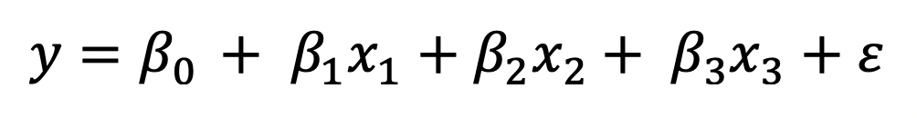
When adding polynomials and interaction terms into an OLS model, the resulting model is still linear. How is that possible? Take a look below. The equation has an interaction term following the intercept and the two main effects.

If we re-express the interaction as a new variable and the coefficient as a new coefficient, the original equation can be re-written as below, which is a linear regression model.

The resulting model is clearly linear:

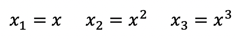
Similarly, polynomial terms can be used in OLS regression, and the resulting model will still be linear. For example, the equation below has second and third degree polynomials.

We can substitute the polynomial terms with the following:
The resulting regression equation is clearly a linear model once again.
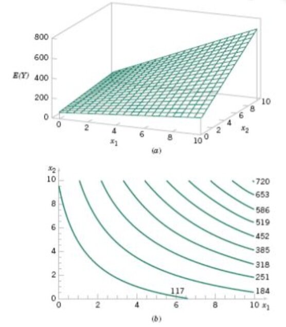
We now established that multiple linear regression models can accommodate the inclusion of interaction effects and polynomials. We can demonstrate this with a three-dimensional plot and its two-dimensional contour plot.

What is a contour plot?
Contour plots display the 3-dimensional relationship in two dimensions, with x- and y-factors (predictors) plotted on the x- and y-scales and response values represented by contours. A contour plot is like a topographical map in which x-, y-, and z-values are plotted instead of longitude, latitude, and elevation.
The surface of the regression is clearly not linear. Still, a regression model with linear parameters will always be linear, even if its generated surface is not. The interaction means that the effect produced by one variable depends on the level of another variable. The plot shows that the impact is a function of both x1 and x2. Further, a quadratic model could take a dome shape , but the value of the regression coefficients may produce a wide array of shapes: but it is still a linear model!
Let’s see how this works with the Boston Housing data. First, the data needed to be loaded and partitioned. Most of the work here was completed with the training data.
#load and partition data
boston= load_boston()
boston_features_df = pd.DataFrame(data=boston.data,columns=boston.feature_names)
boston_target_df = pd.DataFrame(data=boston.target,columns=['MEDV'])

X = boston_features_df.iloc[:,0:13]
y = boston_target_df

#Partition the data
X = boston_features_df
Y = boston_target_df
X_train, X_test, Y_train, Y_test = sklearn.model_selection.train_test_split(X, Y, test_size = 0.20, random_state = 5)
X_train.head()
The following section automatically creates polynomial features and interactions. In fact, all combinations were created! Notice that it is possible to create only interactions and not polynomials but I wanted to do both. This needs to be completed for both the training and test regressors. In this section, I kept all original regressors and the first interaction/polynomial term, which happens to be CRIM^2. Finally, it was necessary to re-index the outcome variable in the training data because the data manipulations of the regressors automatically re-set the index of those data frames. Omitting the re-setting of the Y_train index will result in an error. Later, the whole step will be done in a loop, I just simply wanted to see if the code works.
# Create interaction terms (interaction of each regressor pair + polynomial)
#Interaction terms need to be created in both the test and train datasets
interaction = PolynomialFeatures(degree=2, include_bias=False, interaction_only=False)
interaction
#traning
X_inter = pd.DataFrame(interaction.fit_transform(X_train), columns=interaction.get_feature_names(input_features=boston.feature_names))
X_inter.head(3)

#test
X_inter_t = pd.DataFrame(interaction.fit_transform(X_test), columns=interaction.get_feature_names(input_features=boston.feature_names))
X_inter_t.head(3)

#######################
#create the alternate for dropping all interaction terms Except the first one (the 13th variable in this case)
#This will be used in a loop where the 13th item will be replaced by the 14th, 15th...104th

#train X
X_inter_alt = X_inter.iloc[:, [0, 1, 2, 3, 4, 5, 6, 7, 8, 9, 10, 11, 12, 13]]
print(X_inter_alt.head(3))
print('')
print('')
print('')

#test X
X_inter_t_alt = X_inter_t.iloc[:, [0, 1, 2, 3, 4, 5, 6, 7, 8, 9, 10, 11, 12, 13]]
X_inter_t_alt.head()

#######################

#Since X_inter is used in regression, the index of the that dataset and the outcome variable must be the same
#The index of X_inter was reset during the computation
#Reset the index of Y manually as well
Y_inter=Y_train.reset_index()
Y_inter=Y_inter.drop(['index'], axis=1)
print(Y_inter.head(3))
PolynomialFeatures(degree=2, include_bias=False, interaction_only=False,
                   order='C')
       CRIM    ZN  INDUS  CHAS    NOX     RM    AGE     DIS   RAD    TAX  \
0   1.15172   0.0   8.14   0.0  0.538  5.701   95.0  3.7872   4.0  307.0
1   0.01501  90.0   1.21   1.0  0.401  7.923   24.8  5.8850   1.0  198.0
2  73.53410   0.0  18.10   0.0  0.679  5.957  100.0  1.8026  24.0  666.0

   PTRATIO       B  LSTAT       CRIM^2
0     21.0  358.77  18.35     1.326459
1     13.6  395.52   3.16     0.000225
2     20.2   16.45  20.62  5407.263863


   MEDV
0  13.1
1  50.0
2   8.8
There are 91 combinations of interaction and second degree polynomials in this data. The idea is to place each one of 91 together with the individual regressors (there are 12 of them) one-by-one, fit a model and record statistics about the model. I chose adjusted R squared, which increases only if the newly added regressor improves the model than decreases when the added regressor improves the model less than expected by chance.
The 91 resulting models can be sorted based on their adjusted R squared score. We can then observe, which interaction effect enhances the model, and which are not helping.
The following code takes each of the 91 potential interaction and polynomial terms in a loop, uses statsmodels, calculates and prints all adjusted R squared values. Unfortunately, the printed data does not contain any labels, but I first created an array and transformed it into a data frame.
#print adjusted r squared for each model
#1. Create new datasets where the 13th item changes
#2. print all adjusted r squared stats

for i in range(13,104):
    X_inter_alt2 = X_inter.iloc[:, [0, 1, 2, 3, 4, 5, 6, 7, 8, 9, 10, 11, 12, i]]
    #X_inter_t_alt2 = X_inter.iloc[:, [0, 1, 2, 3, 4, 5, 6, 7, 8, 9, 10, 11, 12, i]] #turned it off - we'd need it if we used stats on test data

    model3 = sm.OLS(Y_inter, sm.add_constant(X_inter_alt2)).fit()
    #Y_pred = model3.predict(sm.add_constant(X_inter_t_alt2)) #turned it off, we do not need predictions on test data
    print_model3 = model3.summary()
    #print(print_model3)

    print(model3.rsquared_adj)

  numbers.append(model3.rsquared_adj)

print(numbers)

#place the array into a data frame
numbers_df=pd.DataFrame(numbers)
numbers_df.head()
| 0 | |
|---|---|
| 0 | 0.728924 |
| 1 | 0.729414 |
| 2 | 0.729445 |
| 3 | 0.740510 |
| 4 | 0.731628 |
Since the individual names of interaction/polynomial terms were available in the original data frame after creating them, I saved them into a data frame and concatenated it with the adjusted R squared values, which can now be sorted and plotted.
#Concatenate the names signifying the 13th variable added to a model with adjusted r squared for each resulting model
#Get row names for all interaction and polynomial features
#first, drop all features that are not interaction or polynomial features
names=X_inter.drop(['CRIM', 'ZN', 'CHAS', 'NOX', 'RM', 'AGE', 'DIS', 'RAD', 'TAX', 'PTRATIO', 'B', 'LSTAT', 'INDUS'], axis=1)
col_heads=pd.DataFrame(list(names))
col_heads

#concatenate col_heads and numbers_df
output=pd.concat([col_heads, numbers_df.reset_index(drop=True)], axis=1)
output.head()

#give columns names otherwise sorting is not possible (by= needs a name to sort on)
output.columns=['names', 'rsquared_adj']
#output.shape

#sort by adjusted r squared: look for items with larger  values
output_sort=output.sort_values(by=['rsquared_adj'])
output_sort
| names | rsquared_adj | |
|---|---|---|
| 22 | ZN PTRATIO | 0.728922 |
| 0 | CRIM^2 | 0.728924 |
| 35 | INDUS LSTAT | 0.728925 |

First few rows of the data frame containing the 91 adjusted R squared statistics.
from pylab import *
x = output_sort['names']
y = output_sort['rsquared_adj']

figure()
plot(x, y, 'r')
xlabel('interaction/polynomial terms')
ylabel('Adjusted R^2 Stat')
title('rsquared_adj')
show()
This graph shows that the adjusted R squared drops quickly until 0.74 and levels off with lower values. Note that the original adjusted R squared of the model without interaction terms was 0.730. Therefore, it is worth considering terms that result in adjusted R squared above 0.74. There aren’t a lot of those!

Now that we identified which terms to consider for fitting a model, we can see how these terms effect the OLS model collectively.
#Select columns with approprite interactions from prior analysis
#X_inter has all variables, polynomials and interactions
selected_df=X_inter[['CRIM', 'ZN', 'INDUS', 'CHAS', 'NOX', 'RM', 'AGE', 'DIS', 'TAX', 'RAD', 'PTRATIO', 'B','LSTAT', 'RM^2', 'RM LSTAT', 'RM TAX', 'RM RAD', 'RM PTRATIO', 'LSTAT^2', 'INDUS RM', 'NOX RM', 'RM AGE', 'RM DIS', 'ZN RM', 'CRIM RM', 'RM B', 'DIS^2', 'CRIM CHAS', 'INDUS DIS']]

#Fit model with new dataset stored in selected_df
import statsmodels.api as sm

model = sm.OLS(Y_inter, sm.add_constant(selected_df)).fit()
print_model = model.summary()
print(print_model)
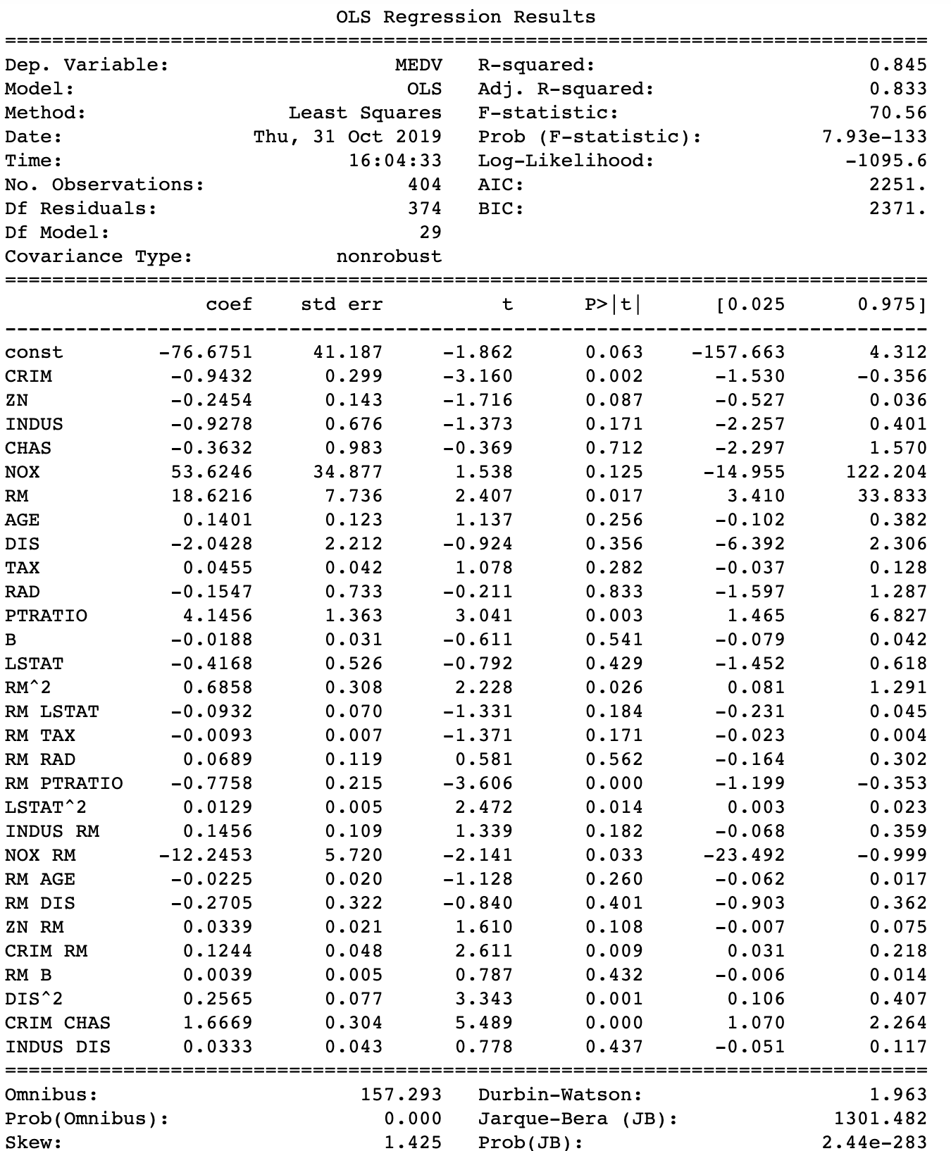
The overall adjusted R squared increased to 0.833, and the AIC/BIC both decreased compared to a model without interactions. The original model’s AIC and BIC was 2432 and 2488 respectively. So now the real work can start by sorting out multicollinearity and play with the model for a better fit and improved accuracy. Still, it seems that introducing interaction and polynomial terms was really worth the effort. As they say, if you torture data, it will confess!