

Multicollinearity

““Cars with flames painted on the hood might get more speeding tickets. Are the flames making the car go fast? No. Certain things just go together. “”
Regressors are orthogonal when there is no linear relationship between them. Unfortunately, linear dependencies frequently exist in real life data, which is referred to as multicollinearity. Multicollinearity could result in significant problems during model fitting. For example, multicollinearity between regressors may result in large variances and covariances for the OLS estimators, which could lead to unstable/poor parameter estimates. In practice, multicollinearity often pushes the parameter estimates higher in absolute value than they really should be. Further, coefficients have been observed to switch signs in multicollinear data. In sum, the multicollinearity should prompt us to question the validity and reliability of the specified model.
Multicollinearity be detected by looking at eigenvalues as well. When multicollinearity exists, at least one of the eigenvalues is close to zero (it suggests minimal variation in the data that is orthogonal with other eigen vectors). Speaking of eigenvalues, their sum equals the number of regressors. Eigenvalues signify the variance in the direction defined by the rotated axis. No variation means limited to no ability to detect trends in the data. Rotation means the defining of new axes by the variances of regressors. Rotation is calculating the weighted averages of standardized regressors. The first new variable accounts for the most variance from a single axis.
Eigen vectors explain the variation in the data orthogonal to other eigen vectors, and the eigen value shows how much variation is in that direction. When eigen values are zero, we need to look for corresponding eigen vectors that are large and the indices of the values show which regressors are collinear.
How to Detect Multicollinearity Easily
Printing and observing bivariate correlations of predictors is not good enough when evaluating the existence of multicollinearity because of potential cross correlation of three or more variables. On the flip side, in certain cases, high correlation between variables does not result in collinearity (e.g. the VIF associated with a variable is not high.)
Instead, one should use variable inflation factor or VIF, which can be computed for each regressor by fitting an OLS model that has the regressor in question as a target variable and all other regressors as features. If a strong relationship exists between the target (e.g. regressor in question) and at least one other regressor, the VIF will be high. What is high? Textbooks usually suggest 5 or 10 as a cutoff value above which the VIF score suggests the presence of multicollinearity. So which one, 5 or 10? If the dataset is very large with a lot of features, a VIF cutoff of 10 is acceptable. Smaller datasets require a more conservative approach where the VIF cutoff may needed to be dropped to 5. I have seen people using an even lower cutoff threshold, and the purpose of the analysis should dictate which threshold to use.
What to do about Multicollinearity
Let me start with a fallacy. Some suggest that standardization helps with multicollinearity. Standardization does not affect the correlation between regressors.
One approach may be the removal of regressors that are correlated. Another may be principal component analysis or PCA. There are other regression methods which may help with the problem such as partial least squares regression or penalized regression methods like ridge or lasso regression. Finally, it may be acceptable to do nothing if the precision of estimating parameters is not that important. So let’s look at multicollinearity in the context of the Boston Housing dataset:
#Import boston dataset from sklearn
import pandas as pd
from sklearn.datasets import load_boston
boston= load_boston()

boston_features_df = pd.DataFrame(data=boston.data,columns=boston.feature_names)
boston_target_df = pd.DataFrame(data=boston.target,columns=['MEDV'])
import sklearn
from sklearn.model_selection import train_test_split #sklearn import does not automatically install sub packages
from sklearn import linear_model
import statsmodels.api as sm
import numpy as np

#Partition the data
#Create training and test datasets
X = boston_features_df
Y = boston_target_df

X_train, X_test, Y_train, Y_test = sklearn.model_selection.train_test_split(X, Y, test_size = 0.20, random_state = 5)
The model fitted below is identical to some of the earlier posts in that it is very rudimentary. It contains all regressors of the Boston Housing data set without any treatment. It is important to look at because I would like to compare how the treatment of multicollinearity changes some of the statistics about the model’s fit.
#Model statistics
#Must add constant for y-intercept
model = sm.OLS(Y_train, sm.add_constant(X_train)).fit()
Y_pred = model.predict(sm.add_constant(X_test))
print_model = model.summary()
print(print_model)
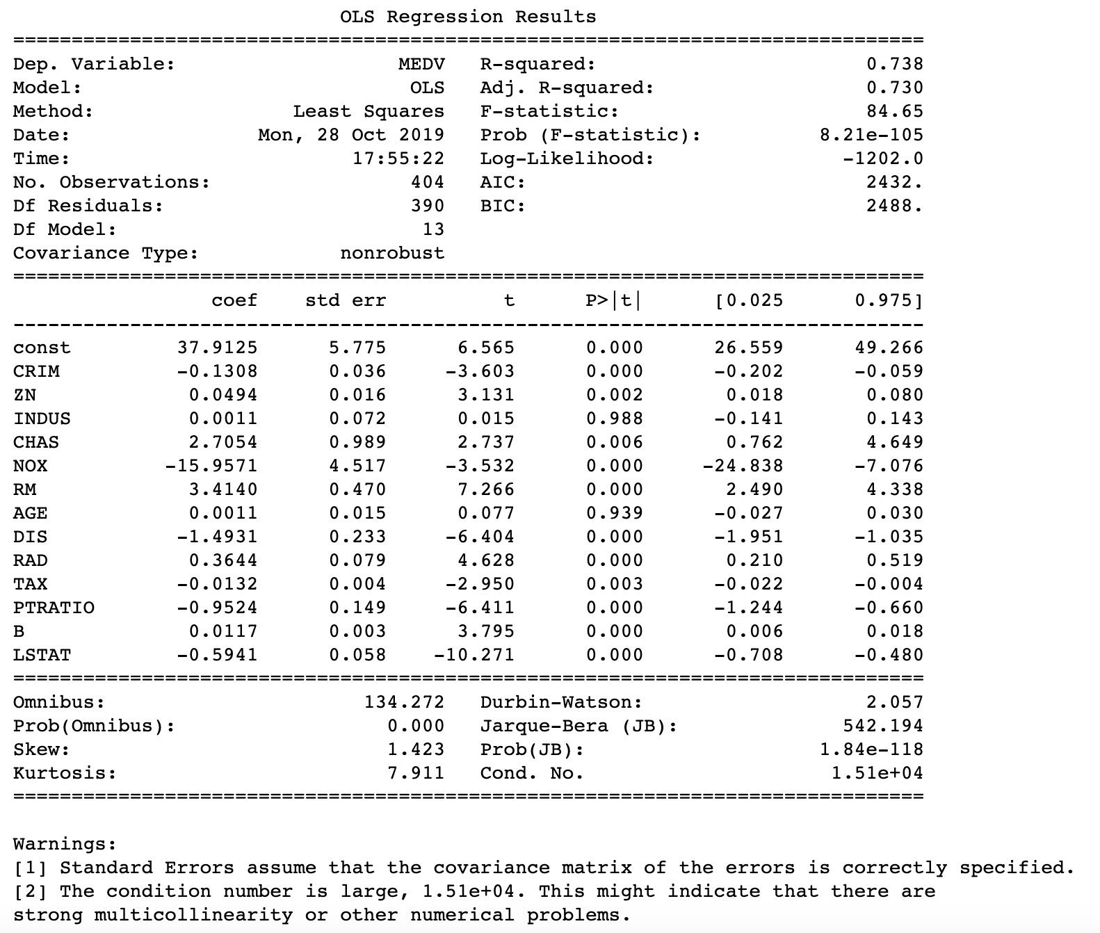
Let’s assess multicollinearity using Variable Inflation Factors. Notice that a constant was added since statsmodels api does not automatically include a y intercept. This very fact caused a lot of headache as I forgot to add the constant many times in the past. Anyway, the print of the VIFs shows that there is collinearity in the data. Both RAD and TAX have VIFs of well above 5.
x_temp = sm.add_constant(X_train)

vif = pd.DataFrame()
vif["VIF Factor"] = [variance_inflation_factor(x_temp.values, i) for i in range(x_temp.values.shape[1])]
vif["features"] = x_temp.columns
print(vif.round(1))
 VIF Factor features
0        578.6    const
1          1.7     CRIM
2          2.4       ZN
3          4.1    INDUS
4          1.1     CHAS
5          4.6      NOX
6          1.8       RM
7          2.9      AGE
8          4.0      DIS
9          8.1      RAD
10         9.8      TAX
11         1.8  PTRATIO
12         1.3        B
13         2.9    LSTAT
In the following code I dropped RAD. Normally, one could start dropping the regressor with the highest VIF. I did start with removing TAX but realized that removing that regressor made the error of the model higher and removing RAD was a much better choice. First, we can observe that removal of RAD fixes all issues with high VIFs.
#ADRESS ISSUES: START WITH ORIGINAL DATASET
boston_new=boston_features_df.drop(['RAD'], axis=1)
boston_new.head()
#Partition the data
#Create training and test datasets
X_1 = boston_new
Y_1 = boston_target_df

X1_train, X1_test, Y1_train, Y1_test = sklearn.model_selection.train_test_split(X_1, Y_1, test_size = 0.20, random_state = 5)

# For each X, calculate VIF and save in dataframe
x_temp = sm.add_constant(X1_train)

vif = pd.DataFrame()
vif["VIF Factor"] = [variance_inflation_factor(x_temp.values, i) for i in range(x_temp.values.shape[1])]
vif["features"] = x_temp.columns
print(vif.round(1))
VIF Factor features
0        532.0    const
1          1.6     CRIM
2          2.3       ZN
3          3.8    INDUS
4          1.1     CHAS
5          4.6      NOX
6          1.8       RM
7          2.9      AGE
8          4.0      DIS
9          3.6      TAX
10         1.8  PTRATIO
11         1.3        B
12         2.9    LSTAT
Now if we fit a new model with the dataset that does not have RAD as a regressor, the model performs somewhat better based on predictions based on test data. While the new model’s AIC and BIC were both slightly higher the calculated test error (MAE) decreased:
model = sm.OLS(Y1_train, sm.add_constant(X1_train)).fit()
Y1_pred = model.predict(sm.add_constant(X1_test))
print_model = model.summary()
print(print_model)

import sklearn
from sklearn import metrics

print('Mean Absolute Error ( Base):', metrics.mean_absolute_error(Y_test, Y_pred))
print('')
print('Mean Absolute Error (Not collinear):', metrics.mean_absolute_error(Y_test, Y1_pred))
Mean Absolute Error ( Base): 3.213270495842386

Mean Absolute Error (Not collinear): 3.1398352911129916


