Manatee Data: Simple OLS Regression

Simple Ordinary Least Squares Regression with statsmodels. api

““Regression lives on, not because of the unavailability of a better option but because of the inertia and fear of change. A known devil is NOT better than an unknown one because there is a fifty percent chance that unknown may not be a devil at all.””

— EverSkeptic

I am continuing the discussion about general linear models. In one of the prior post, I demonstrated how simple linear regression works. I looked at individual observations and computed several items including the slope, the y intercept and the coefficient of determination. I also tested the significance of the coefficient and that of the model suing t statistic and F statistic, respectively.

In this writing, I wanted to focus on computing the intercept and regression coefficient using statstmodels. api and statsmodels.formula.api. As you’ll see later the difference between the two is that one needs manual insertion of an intercept, while the other does not.

The first task is the same as in the manual regression example. I created a data set from data I collected from the Internet. The manatee death data came from the Florida Fish and Wildlife Conservation Commission and the boat registration data was sourced from the Florida from the Department of Highway Safety and Motor Vehicles (FLHSMV). An explanation of how the data was gathered and what it actually represents is available from Manatee Data: General Linear

<#CREATE LISTS
year=[2000,2001,2002,2003,2004,2005,2006, 2007, 2008, 2009, 2010, 2011, 2012, 2013, 2014, 2015, 2016, 2017]
boat_deaths=[78,81,95,73,69,79,92,73,90,97,83,88,82,73,69,86,106,111]
manatee_deaths=[272, 325, 305, 380, 276, 396, 417, 317, 337, 429, 766, 453, 392, 830, 371, 405, 520, 538]

#Number of vessels by class
#Only vessels equipped with an EPIRB (Emergency Position, Indicationg Radio Becon) considered by class
#p indicates pleasure and c indicates commercial

classA1_p=[137301,148860,151175, 153777,154673, 159064,163463, 165424, 159055, 157214, 149968,144134,138975,136879,136860,139957,143490,146747]
classA1_c=[1243, 1384, 1432, 1435,1360,1263,1231,1215, 1268, 1105, 1093, 1066, 1081,1141,1214,1235,1286,1304]
classA2_p=[231836,243178,240799,237163,230638,228821,225801, 221348, 228829, 209058,198589, 191071, 184530,180914,178379,178092,176956,174154]
classA2_c=[5178,5518,5256, 5016,4789, 4554, 4411, 4346, 4555, 4122, 4113, 4166, 4077,4035,4075,4084,3964,3854]
class1_p=[397101,428404,443393, 457661,466122,485192, 495592, 499110, 485168, 480232,460579, 455430, 447638,446920,450335,460125,470587,480158]
class1_c=[13906, 14697,14468, 14355,13974,13967,13757, 13690, 13990, 13598,13930, 14064,14103, 14158,14324,14526,14458,14274]
class2_p=[59103, 64710,67816, 70944,73395,78028,80300, 81824, 78040, 78823, 76840, 75571, 74877,75271,76299,78510,80750,83108]
class2_c=[4892, 5175, 5132, 5077, 4885,4945, 4803, 4718, 4929, 4552, 4569, 4596, 4557,4567,4539,4573,4533,4562]
class3_p=[10430,10874,11810, 12086,12472,13293,13569, 13669, 13290, 13015, 12845, 12898, 12928,13265,13763,14349,15003,15566]
class3_c=[2218,2194,2154, 2099,2015, 1943,1890, 1817, 1945,1667, 1658, 1641, 1548,1539,1524,1513,1492,1492]
class4_p=[499,553,601, 638, 666,744,776, 783, 742, 758, 807, 926, 1032,1153,1287,1444,1561,1670]
class4_c=[494,514, 507, 483, 463,455,417, 386,  454, 349, 329, 299, 290,271,270,263,250,255]
class5_p=[43,40,43, 42,58,68,75, 91, 67, 58, 59,58,63,75,92,117,115,131]
class5_c=[25, 31, 35, 32,29,27,33, 33, 27, 30,27,81, 77,77,84,84,82,82]

# CREATE A LIST OF LISTS
manatee_data=[year, boat_deaths, manatee_deaths, classA1_p, classA1_c, classA2_p, classA2_c, class1_p, class1_c, class2_p, class2_c, class3_p, class3_c, class4_p, class4_c, class5_p, class5_c]

# CREATE DATA FRAME USING PANDAS
# FIRST IMPORT PANDAS
import pandas as pd
manatee_data_df = pd.DataFrame(manatee_data) 
#TRANSPOSE DATAFRAME
manatee_data_df = manatee_data_df.T
#NAME COLUMNS
manatee_data_df.columns = ['year', 'boat_deaths', 'manatee_deaths', 'classA1_p', 'classA1_c', 'classA2_p', 
                     'classA2_c', 'class1_p', 'class1_c', 'class2_p', 'class2_c', 'class3_p', 'class3_c', 
                     'class4_p', 'class4_c', 'class5_p', 'class5_c']

#ADD ALL BOAT TYPES AND CREATE A SINGLE VALUE
manatee_data_df['all_boats']=manatee_data_df['classA1_p']+manatee_data_df['classA1_c']+manatee_data_df['classA2_p']+manatee_data_df['classA2_c']+manatee_data_df['class1_p']+manatee_data_df['class1_c']+manatee_data_df['class2_p']+manatee_data_df['class2_c']+manatee_data_df['class3_p']+manatee_data_df['class3_c']+manatee_data_df['class4_p']+manatee_data_df['class4_c']+manatee_data_df['class5_p']+manatee_data_df['class5_c']
manatee_data_df.head(5)
#create x and y values
x=manatee_data_df['all_boats']
y=manatee_data_df['boat_deaths']

The statsmodel.api allows us to fit an Ordinary Least Squares model. This is a linear model that estimates the intercept and regression coefficient. These parameters are chosen and estimated by the method of least squares, e.g. we minimize the sum of squared differences between actual observations of the dependent variable vs. predicted values of the dependent variable. The predictions are based on a linear function.

When visualizing OLS, it is the sum of squared distances between data points and the regression line, parallel to the y axis (axis of the dependent variable). When the sum of the distances is small, the model is considered a better representation/fit of the data.

Statsmodels api

When estimating parameters with this method, be sure to add a constant that will account for the y intercept. The statsmodels OLS estimator does not automatically come with the constant. Also, we must ensure that the values in the data frame equal 1. I have seen people trying to add 0s but the package will show an error.

#Use statsmodels package for simple regression
import numpy as np
import statsmodels.api as sm

#Add constant term 
#OLS statsmodels doesn't have intercept 
#Must use formulas
x_1=sm.add_constant(x)
x_1.head()

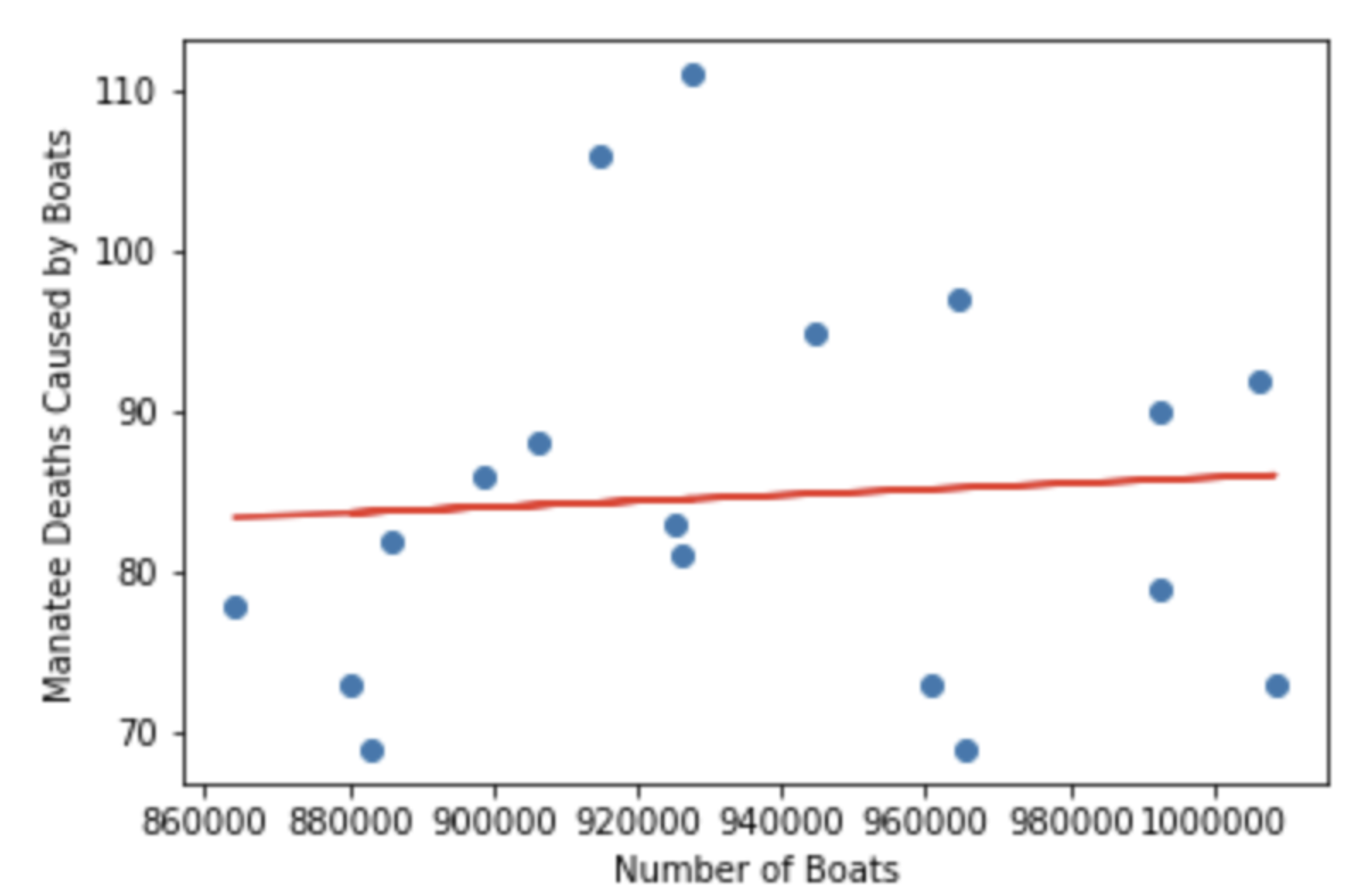
When I ran the statsmodels OLS package, I managed to reproduce the exact y intercept and regression coefficient I got when I did the work manually (y intercept: 67.580618, regression coefficient: 0.000018.) One must print results.params to get the above mentioned parameters. The plot of observations and regression line look the same as well, which is very reassuring for what I tried to accomplish earlier.

model = sm.OLS(y,x_1)
results = model.fit()
results
print(results.params)

import matplotlib.pyplot as plt
y_hat=results.predict(x_1)
plt.scatter(x,y)
plt.xlabel("Number of Boats")
plt.ylabel("Manatee Deaths Caused by Boats")
plt.plot(x,y_hat, "r")
plt.show()

statsmodels.formula.api

Now, we can accomplish the exact same result by using statsmodels.formula.api. In this case, we do not have to add a constant, as this module does have a built in y-intercept.

manatee_df=pd.DataFrame(x)
manatee_df.rename(columns={'all_boats':'x'}, inplace=True)
manatee_df['y']=y
manatee_df.head()

results_formula = sm1.ols(formula='y ~ x', data=manatee_df).fit()
print(results_formula.params)

I am very please to see that this method also reproduces the same parameters (y intercept: 67.580618, regression coefficient: 0.000018.)

While the method of fitting a simple OLS model is simple, I do think it is important to understand what we are doing during the fitting of these models before moving onto more complicated things. I hope I managed to describe the basics of regression modeling.