
Linear and Quadratic Discriminant Analysis

““The problem with the Internet is that it gives you everything - reliable material and crazy material. So the problem becomes, how do you discriminate?” ”
Revised on Feb. 10, 2020
Table of Contents:
In order to arrive at the most accurate prediction, machine learning models are built, tuned and compared against each other. The reader can get can click on the links below to assess the models or sections of the exercise. Each section has a short explanation of theory, and a description of applied machine learning with Python:
LDA/QDA/Naive Bayes Classifier (Current Blog)
Ensemble Learning
Objectives:
This blog is part of a series of models showcasing applied machine learning models in a classification setting. By clicking on any of the tabs below, the reader can navigate to other methods of analysis applied to the same data. This was designed so that one could see what a data scientist would do from soup to nuts when faced with a problem like the one presented here. Note that the overall focus of this blog is Linear and Quadratic Discriminant Analysis as well as the Naive Bayes Classifier.
Learn about Bayes’ Theorem and its application in making class predictions;
Get introduced to Linear Discriminant Analysis;
Gain familiarity with Quadratic Discriminant Analysis;
Understand the conceptual and mathematical differences between LDA, QDA and the Naive Bayes Classifier;
Find out how to use Sci-Kit Learn to fit LDA, QDA, NBC;
Learn how to tune parameters with GridSeachCV(); and
Refresh how to gauge the accuracy of classification models
ROC Curves
Confusion Matrix
Accuracy score, F1, Precision, Recall
Bayes’ Theorem for Classification:
We can classify an observation into one of K classes (K≥ 2), and K can take unordered and distinct values according to Introduction to Statistical Learning (James et al.). Click for more. When classifying observations, one can use Bayes’ Theorem, which describes the probability of an event, based on prior knowledge of conditions that might be related to the event. For example, if getting into a car accident is related to the driver’s prior history of speeding, then assessing the probability of getting into a car accident in the future can be done with higher accuracy if the analyst has information about the number of speeding tickets vs. when the analyst does not have access to the history of an individual’s driving record. The mathematical notation of Bayes’ Theorem is

where A and B are events and P(B) ≠ 0.
P(A| B)} is a conditional probability: the likelihood of event A occurring given that B is true.
P(B|A) is also a conditional probability: the likelihood of event B occurring given that A is true.
P(A)} and P(B) are the probabilities of observing A and B respectively; they are known as the marginal probability.
Bayes’ Theorem can be rewritten as below given that πk(the prior or posterior probability that an observation belongs to the kth class, e.g. if we randomly choose an observation, it comes from the kth class. Also, the density function of X for an observation comes from the kth class is fk(x) ≡ Pr(X = x|Y = k).

Instead of directly computing pk(X) , we can simply use πk(the prior or posterior probability that an observation belongs to the kth class) and the fk(x), e.g. density function: fk(x) ≡ Pr(X = x|Y = k). This means that we can compute the probability that an observation belongs to a certain class given the predictor value for the observation. The Bayes classifier classifies an observation to the class for which fk(x) is the largest and has the lowest error rate compared to all other classifiers. So if fk(x) is large than the probability that an observation belongs to the kth class is high. If fk(x) is small, than the probability that an observation fk(x) belongs to the same kth class is minimal. In analytics, we must estimate fk(x) based on pk(x), which is called the posterior probability that an observation belongs to the kth class.
Linear Discriminant Analysis:
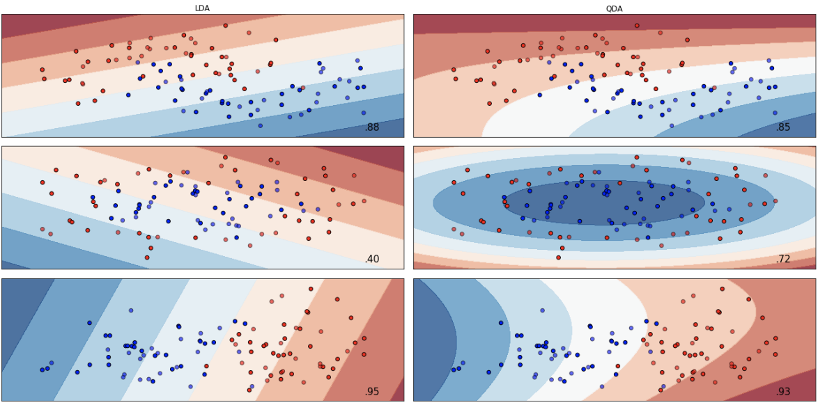
Linear Discriminant Analysis (LDA) is a method that is designed to separate two (or more) classes of observations based on a linear combination of features. The linear designation is the result of the discriminant functions being linear.
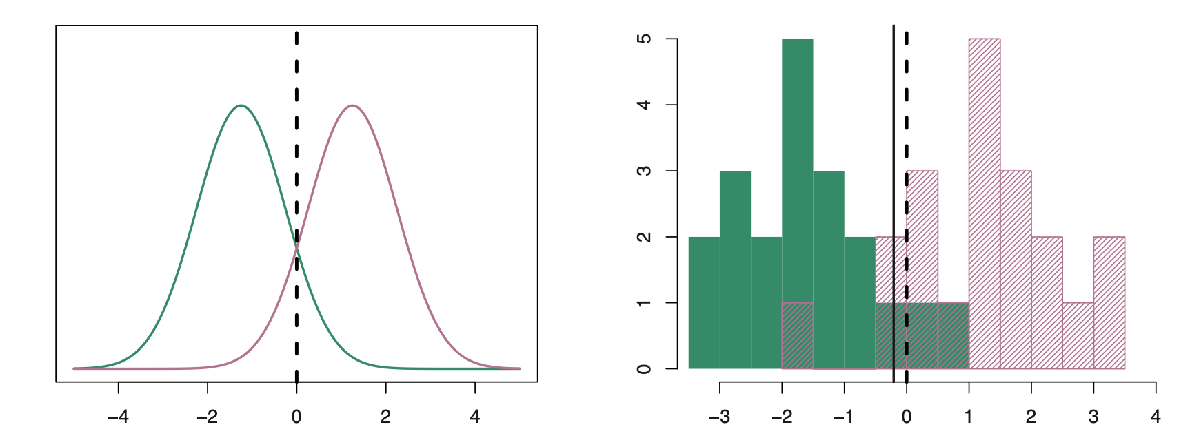
The image above shows two Gaussian density functions. (Source: Introduction to Statistical Learning - James et al.) Click for more. The dashed vertical line shows the decision boundary. The right side shows histograms of randomly chosen observations. The dashed line again is the Bayesian decision boundary. The solid vertical line is the LDA decision boundary estimated from the training data. When the Bayesian decision boundary and the LDA decision boundary are close, the model is considered to perform well.
LDA is used to estimate πkusing the proportion of the training observations that belong to the kth class. In this example there is only one regressor (p=the number of regressors). When multiple regressors are used, then observations are assumed to be drown from a multivariate Gaussian distribution.
Quadratic Discriminant Analysis:
Quadratic Discriminant Analysis (QDA) is similar to LDA based on the fact that there is an assumption of the observations being drawn form a normal distribution. The difference is that QDA assumes that each class has its own covariance matrix, while LDA does not.
QDA classifier uses several parameters (Σk, μk, and π k) to determine in which class should an observation be classified. Whether we use QDA or LDA depends on the bias-variance tradeoff. LDA is less flexible with lower variance. However, in LDA, observations share a common covariance matrix, resulting in higher bias.
ANALYTICS WITH With Python:
LDA: Sci-Kit Learn uses a classifier with a linear decision boundary, generated by fitting class conditional densities to the data and using Bayes’ rule. The model fits a Gaussian density to each class, assuming that all classes share the same covariance matrix. (Source: Sci-Kit Learn - Click for more)
QDA: Quadratic Discriminant Analysis
Sci-Kit Learn uses a classifier with a quadratic decision boundary based on fitted conditional densities as described by Bayes’ Theorem. Each class is fitted with a Gaussian density. (Source: Sci-Kit Learn - Click for more)
The first block loads all necessary libraries, creates the regressors and the dependent variable required by sklearn. Finally, the data set is partitioned into train and test sets.
import numpy as np
import pandas as pd
import matplotlib.pyplot as plt

import sklearn
from sklearn.preprocessing import PolynomialFeatures
from sklearn.preprocessing import StandardScaler

from sklearn.model_selection import train_test_split
from sklearn.model_selection import GridSearchCV
from sklearn import metrics
from sklearn.metrics import confusion_matrix
from sklearn.metrics import classification_report
from sklearn.metrics import roc_auc_score

import warnings

from sklearn.discriminant_analysis import LinearDiscriminantAnalysis
from sklearn.discriminant_analysis import QuadraticDiscriminantAnalysis
from sklearn.naive_bayes import GaussianNB

#read csv file
charity_df = pd.read_csv('charity.csv')
charity_df.head(3)

charity_df = pd.read_csv('charity.csv') #read csv file
charity_df=charity_df.dropna() #remove all lines with missing observations
charity_df = charity_df.drop('damt', axis=1) #drop damt

#Create regressors and dependent variable
X = charity_df.drop(['donr', 'ID'], axis=1) #note that donr was dropped from X because it is the dependent variable
y = charity_df['donr']

#Create training and test datasets
X_train, X_test, y_train, y_test = sklearn.model_selection.train_test_split(X, y, test_size = 0.20, random_state = 5)
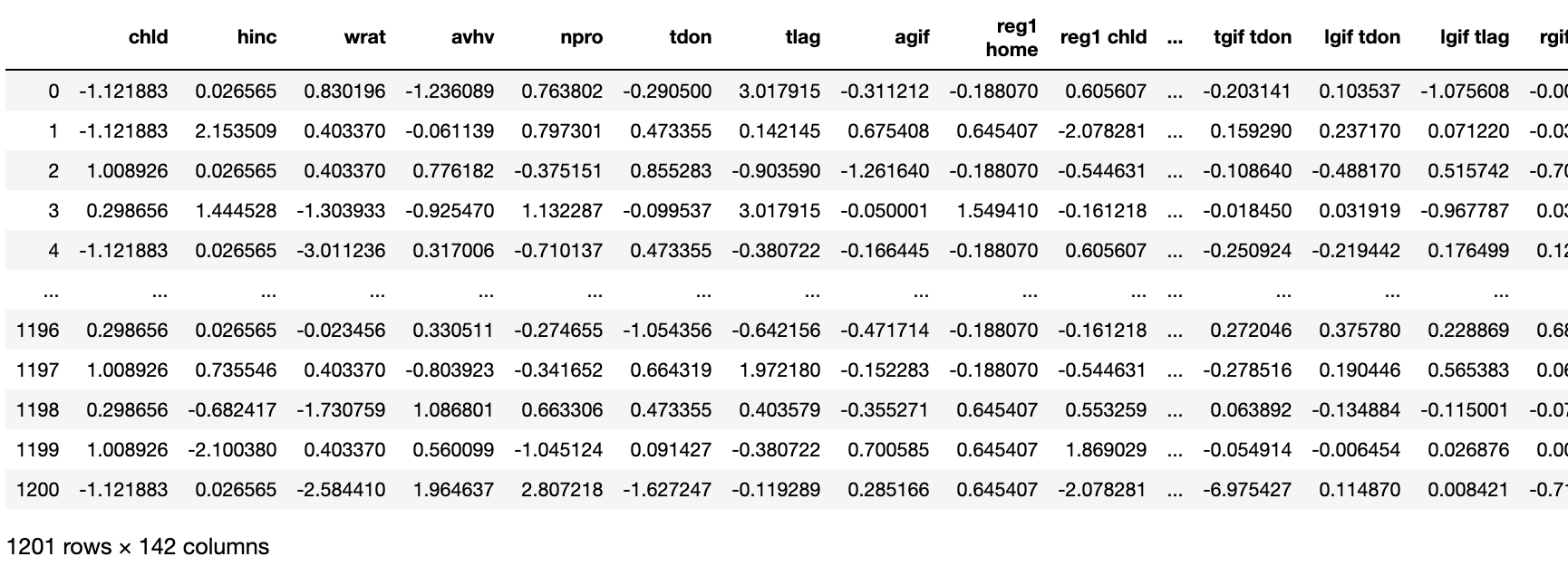
Since we are charged with creating the best model possible, let us create new features. Here, we’ll create second order polynomials and interaction terms, and separately, we create third order polynomials and third degree interaction terms. Creation of these terms will bring up some issues but will spend more time on that in a bit. For now, just notice that creating third order polynomials increased our column count from 23 to 1,539.
# Create interaction terms (interaction of each regressor pair + polynomial)
#Interaction terms need to be created in both the test and train datasets
interaction2 = PolynomialFeatures(degree=2, include_bias=False, interaction_only=False, order='C') #second degree
interaction3 = PolynomialFeatures(degree=3, include_bias=False, interaction_only=False, order='C') #third degree

#traning
X_train_2 = pd.DataFrame(interaction2.fit_transform(X_train), columns=interaction2.get_feature_names(input_features=X_train.columns))
X_train_3 = pd.DataFrame(interaction3.fit_transform(X_train), columns=interaction3.get_feature_names(input_features=X_train.columns))

X_train_2.head()

#test
X_test_2 = pd.DataFrame(interaction2.fit_transform(X_test), columns=interaction2.get_feature_names(input_features=X_train.columns))
X_test_3 = pd.DataFrame(interaction3.fit_transform(X_test), columns=interaction3.get_feature_names(input_features=X_train.columns))

X_test_3.head()

When fitting LDA models, standardizing or scaling is a good idea. There are several articles out there explaining why standardizing is a must. Here we have to remember to standardize all of our data sets.
#############################
## Standardize all datasets
#############################
scaler = StandardScaler(copy=True, with_mean=True, with_std=True)

#Standardize the training sets: 1st, 2nd and 3rd order polynomials

X_train=pd.DataFrame(scaler.fit_transform(X_train), columns=X_train.columns)
X_train_2=pd.DataFrame(scaler.fit_transform(X_train_2), columns=X_train_2.columns)
X_train_3=pd.DataFrame(scaler.fit_transform(X_train_3), columns=X_train_3.columns)

#Standardize the test sets: 1st, 2nd and 3rd order polynomials

X_test=pd.DataFrame(scaler.fit_transform(X_test), columns=X_test.columns)
X_test_2=pd.DataFrame(scaler.fit_transform(X_test_2), columns=X_test_2.columns)
X_test_3=pd.DataFrame(scaler.fit_transform(X_test_3), columns=X_test_3.columns)
X_train.head()

Since we created interaction terms and polynomials, multicollinearity will certainly be an issue. Here, we check if multicollinearity exists in the original data set, and then we go through the newly created two data sets containing second and third degree polynomials the same way. We make use of VIF and identify all variables with a VIF of greater than 5. We simply will eliminate these variables from the analysis.
################################
## Deal with multicollinearity
################################

import statsmodels.api as sm
from statsmodels.stats.outliers_influence import variance_inflation_factor

#1st order polynomial ######################
x_temp_train1 = sm.add_constant(X_train)
vif_train1 = pd.DataFrame()
vif_train1["VIF Factor"] = [variance_inflation_factor(x_temp_train1.values, i) for i in range(x_temp_train1.values.shape[1])]
vif_train1["features"] = x_temp_train1.columns
pd.set_option('display.max_rows', 300)
print(vif_train1.round(1))

vif_train1_a=vif_train1[vif_train1["VIF Factor"]<5.0] #identify all variables wit VIF less then 5 and keep
#print(vif2.round(1))

feat_list=vif_train1_a["features"].tolist()  #save desired features to list
feat_list.remove(feat_list[0])
print(feat_list)

X_train=X_train[feat_list] #keep features on feature list only, drop all other features for train
X_test=X_test[feat_list]   #keep features on feature list only, drop all other features for test

   VIF Factor features
0          1.0    const
1          1.6     reg1
2          1.8     reg2
3          1.4     reg3
4          1.5     reg4
5          1.0     home
6          1.0     chld
7          1.0     hinc
8          1.0     genf
9          1.0     wrat
10         2.3     avhv
11         2.4     incm
12         1.9     plow
13         2.2     npro
14         2.3     tgif
15         2.3     lgif
16         2.7     rgif
17         1.0     tdon
18         1.0     tlag
19         2.2     agif
['reg1', 'reg2', 'reg3', 'reg4', 'home', 'chld', 'hinc', 'genf', 'wrat', 'avhv', 'incm', 'plow', 'npro', 'tgif', 'lgif', 'rgif', 'tdon', 'tlag', 'agif']

And now the painful task of eliminating variables begins. This may be a slow process if the dataset is large. Think about it: We need to create a matrix of correlations among all variables.
#2nd order polynomial ####################
x_temp_train2 = sm.add_constant(X_train_2)
vif_train2 = pd.DataFrame()
vif_train2["VIF Factor"] = [variance_inflation_factor(x_temp_train2.values, i) for i in range(x_temp_train2.values.shape[1])]
vif_train2["features"] = x_temp_train2.columns
pd.set_option('display.max_rows', 300)
#print(vif_train1.round(1))

vif_train2_a=vif_train2[vif_train2["VIF Factor"]<5.0]
#print(vif2.round(1))

feat_list2=vif_train2_a["features"].tolist()
feat_list2.remove(feat_list2[0])
print(feat_list2)

X_train_2=X_train_2[feat_list2] #keep features on feature list only, drop all other features for train
X_test_2=X_test_2[feat_list2]   #keep features on feature list only, drop all other features for test
X_test_2

['chld', 'hinc', 'wrat', 'avhv', 'npro', 'tdon', 'tlag', 'agif', 'reg1 home', 'reg1 chld', 'reg1 hinc', 'reg1 genf', 'reg1 wrat', 'reg1 avhv', 'reg1 incm', 'reg1 plow', 'reg1 npro', 'reg1 tgif', 'reg1 rgif', 'reg1 tdon', 'reg1 tlag', 'reg1 agif', 'reg2 home', 'reg2 chld', 'reg2 hinc', 'reg2 genf', 'reg2 wrat', 'reg2 avhv', 'reg2 incm', 'reg2 plow', 'reg2 npro', 'reg2 tdon', 'reg2 tlag', 'reg3 home', 'reg3 chld', 'reg3 hinc', 'reg3 genf', 'reg3 wrat', 'reg3 avhv', 'reg3 incm', 'reg3 plow', 'reg3 npro', 'reg3 tgif', 'reg3 rgif', 'reg3 tdon', 'reg3 tlag', 'reg3 agif', 'reg4 home', 'reg4 chld', 'reg4 hinc', 'reg4 genf', 'reg4 wrat', 'reg4 avhv', 'reg4 incm', 'reg4 plow', 'reg4 npro', 'reg4 tgif', 'reg4 tdon', 'reg4 tlag', 'reg4 agif', 'home chld', 'home hinc', 'home genf', 'home wrat', 'home avhv', 'home incm', 'home plow', 'home npro', 'home tgif', 'home lgif', 'home rgif', 'home tdon', 'home tlag', 'home agif', 'chld^2', 'chld hinc', 'chld genf', 'chld wrat', 'chld avhv', 'chld incm', 'chld plow', 'chld npro', 'chld tgif', 'chld lgif', 'chld rgif', 'chld tdon', 'chld tlag', 'chld agif', 'hinc^2', 'hinc genf', 'hinc wrat', 'hinc avhv', 'hinc incm', 'hinc plow', 'hinc npro', 'hinc tgif', 'hinc lgif', 'hinc rgif', 'hinc tdon', 'hinc tlag', 'hinc agif', 'genf wrat', 'genf avhv', 'genf incm', 'genf plow', 'genf npro', 'genf tgif', 'genf lgif', 'genf rgif', 'genf tdon', 'genf tlag', 'genf agif', 'wrat^2', 'wrat avhv', 'wrat incm', 'wrat plow', 'wrat npro', 'wrat tgif', 'wrat lgif', 'wrat rgif', 'wrat tdon', 'wrat tlag', 'wrat agif', 'avhv tdon', 'avhv tlag', 'incm tdon', 'incm tlag', 'plow tdon', 'plow tlag', 'npro^2', 'npro tdon', 'npro tlag', 'tgif tdon', 'lgif tdon', 'lgif tlag', 'rgif tdon', 'rgif tlag', 'tdon^2', 'tdon tlag', 'tdon agif', 'tlag^2', 'tlag agif']
#3rd order polynomial ####################
x_temp_train3 = sm.add_constant(X_train_3)
vif_train3 = pd.DataFrame()
vif_train3["VIF Factor"] = [variance_inflation_factor(x_temp_train3.values, i) for i in range(x_temp_train3.values.shape[1])]
vif_train3["features"] = x_temp_train3.columns
pd.set_option('display.max_rows', 300)
#print(vif_train3.round(1))

vif_train3_a=vif_train3[vif_train3["VIF Factor"]<5.0]
#print(vif3.round(1))

feat_list3=vif_train3_a["features"].tolist()
feat_list3.remove(feat_list3[0])
print(feat_list3)

X_train_3=X_train_3[feat_list3] #keep features on feature list only, drop all other features for train
X_test_3=X_test_3[feat_list3]   #keep features on feature list only, drop all other features for test

                                                      ['chld', 'hinc', 'wrat', 'npro', 'tdon', 'tlag', 'agif', 'reg1 home', 'reg1 chld', 'reg1 hinc', 'reg1 genf', 'reg1 wrat', 'reg1 plow', 'reg1 npro', 'reg1 tgif', 'reg1 rgif', 'reg1 tdon', 'reg1 tlag', 'reg1 agif', 'reg2 home', 'reg2 chld', 'reg2 hinc', 'reg2 genf', 'reg2 wrat', 'reg2 plow', 'reg2 npro', 'reg2 tdon', 'reg2 tlag', 'reg3 home', 'reg3 chld', 'reg3 hinc', 'reg3 genf', 'reg3 wrat', 'reg3 plow', 'reg3 npro', 'reg3 tgif', 'reg3 rgif', 'reg3 tdon', 'reg3 tlag', 'reg3 agif', 'reg4 home', 'reg4 chld', 'reg4 hinc', 'reg4 genf', 'reg4 wrat', 'reg4 plow', 'reg4 npro', 'reg4 tgif', 'reg4 tdon', 'reg4 tlag', 'reg4 agif', 'home chld', 'home hinc', 'home genf', 'home wrat', 'home avhv', 'home incm', 'home plow', 'home npro', 'home tgif', 'home lgif', 'home rgif', 'home tdon', 'home tlag', 'home agif', 'chld^2', 'chld hinc', 'chld genf', 'chld wrat', 'chld avhv', 'chld incm', 'chld plow', 'chld npro', 'chld tgif', 'chld lgif', 'chld rgif', 'chld tdon', 'chld tlag', 'chld agif', 'hinc^2', 'hinc genf', 'hinc wrat', 'hinc avhv', 'hinc incm', 'hinc plow', 'hinc npro', 'hinc tgif', 'hinc lgif', 'hinc rgif', 'hinc tdon', 'hinc tlag', 'hinc agif', 'genf wrat', 'genf avhv', 'genf incm', 'genf plow', 'genf npro', 'genf tgif', 'genf lgif', 'genf rgif', 'genf tdon', 'genf tlag', 'genf agif', 'wrat^2', 'wrat avhv', 'wrat incm', 'wrat plow', 'wrat npro', 'wrat tgif', 'wrat lgif', 'wrat rgif', 'wrat tdon', 'wrat tlag', 'wrat agif', 'avhv tdon', 'avhv tlag', 'incm tdon', 'plow tdon', 'plow tlag', 'npro^2', 'npro tdon', 'npro tlag', 'tgif tdon', 'lgif tdon', 'lgif tlag', 'rgif tdon', 'rgif tlag', 'tdon^2', 'tdon tlag', 'tdon agif', 'tlag^2', 'tlag agif']

In both cases, the number of variables was reduced significantly. The second order polynomial file now has only 142 features, while the third order polynomial file contains only 148 features vs. the 1,539 we started with. We are ready to fit some models.
Parameter Tuning:
Our first task is to fit a generic LDA model without any parameters tuned for two reasons: understand code structure and get a baseline accuracy. For fitting, we are using the first degree polynomial, e.g. the original dataset.
#Default LDA model without any tuning - base metric
LDA_model_default = LinearDiscriminantAnalysis()
LDA_model_default.fit(X_train, y_train)
y_pred_LDA_default =LDA_model_default.predict(X_test)
So let us try to tune the parameters of the LDA model. A list of tunable parameters can be found on the Scikit-Learn Linear Discriminant Analysis Page (Please click to navigate). There are three different solvers one can try, but one of them (svd) does not work with shrinkage. As a result, the cross validation routines using GridSearchCV were separated in the code below for the two solver that work with shrinkage vs. the the one that does not. The shrinkage parameter can be tuned or set to auto as well. Nuanced difference but it does impact the final model selected. In the final run shown here, the solver type and n_components were tuned.
Also, please note that GridSearchCV itself has a myriad of options. For selection of champion models, accuracy was chosen as a decision metric. Documentation of GridSearchCV is available by clicking here.
#Parameter tuning with GridSearchCV

#######################
### LDA  - lsqr & eigen
#######################

estimator_1 = LinearDiscriminantAnalysis(shrinkage='auto')
parameters_1 = {
    'solver': ('lsqr','eigen'),  #note svd does not run with shrinkage and models using it will be tuned separately
    'n_components': (1,5,1),
                   }
# with GridSearch
grid_search_lda_A = GridSearchCV(
    estimator=estimator_1,
    param_grid=parameters_1,
    scoring = 'accuracy',
    n_jobs = -1,
    cv = 5
)
lda_A1=grid_search_lda_A.fit(X_train, y_train)
y_pred_1 =lda_A1.predict(X_test)

lda_A2=grid_search_lda_A.fit(X_train_2, y_train)
y_pred_2 =lda_A2.predict(X_test_2)

lda_A3=grid_search_lda_A.fit(X_train_3, y_train)
y_pred_3 =lda_A3.predict(X_test_3)
Predictions were made with all three datasets (e.g. 1st, 2nd and 3rd degree polynomial datasets.), which will be used later for assessment of model accuracy. Below is the tuning of the svd model followed by model fitting and predicting outcomes based on test data.
#Parameter tuning with GridSearchCV

#######################
### LDA  - svd
#######################

estimator_2 = LinearDiscriminantAnalysis(solver='svd', )#note svd does not run with shrinkage and models using it will be tuned separately
parameters_2 = {
    'n_components': (0,5,1),
    'store_covariance' :(True, False),
                   }
# with GridSearch
grid_search_lda_B = GridSearchCV(
    estimator=estimator_2,
    param_grid=parameters_2,
    scoring = 'accuracy',
    n_jobs = -1,
    cv = 5
)
lda_B1=grid_search_lda_B.fit(X_train, y_train)
y_pred_4 =lda_B1.predict(X_test)

lda_B2=grid_search_lda_B.fit(X_train_2, y_train)
y_pred_5 =lda_B2.predict(X_test_2)

lda_B3=grid_search_lda_B.fit(X_train_3, y_train)
y_pred_6 =lda_B3.predict(X_test_3)
Quadratic Discriminant Analysis:
The next section is focused on QDA. A list of tunable parameters is available by clicking here. GridSearchCV was once again used for parameter tuning, and the final exercise looked at the tuning of three parameters.
#Base QDA Without any tuning
QDA_model_default = QuadraticDiscriminantAnalysis()
QDA_model_default.fit(X_train, y_train)
y_pred_QDA_default =QDA_model_default.predict(X_test)

#Parameter tuning with GridSearchCV
#######################
### QDA
#######################

estimator_3 = QuadraticDiscriminantAnalysis()
parameters_3 = {
    'reg_param': (0.00001, 0.0001, 0.001,0.01, 0.1),
    'store_covariance': (True, False),
    'tol': (0.0001, 0.001,0.01, 0.1),
                   }
# with GridSearch
grid_search_qda = GridSearchCV(
    estimator=estimator_3,
    param_grid=parameters_3,
    scoring = 'accuracy',
    n_jobs = -1,
    cv = 5
)
qda_1=grid_search_qda.fit(X_train, y_train)
y_pred_7 =qda_1.predict(X_test)

qda_2=grid_search_qda.fit(X_train_2, y_train)
y_pred_8 =qda_2.predict(X_test_2)

qda_3=grid_search_qda.fit(X_train_3, y_train)
y_pred_9 =qda_3.predict(X_test_3)
Naive Bayes Classifier:
Finally, we fitted a Naive Bayes Classifier with the exact same GridSearchCV approach as the one used by LDA and QDA. NBA can also be tuned, and the tunable parameter list can be reached by clicking here.
#Parameter tuning with GridSearchCV

##########################
### QGaussian Naive Bayes
##########################


estimator_4 = GaussianNB()
parameters_4 = {
    'var_smoothing': (0,1e-9,1e-7, 1e-5),
                   }
# with GridSearch
grid_search_gnb = GridSearchCV(
    estimator=estimator_4,
    param_grid=parameters_4,
    scoring = 'accuracy',
    n_jobs = -1,
    cv = 5
)
gnb_1=grid_search_gnb.fit(X_train, y_train)
y_pred_10 =gnb_1.predict(X_test)

gnb_2=grid_search_gnb.fit(X_train_2, y_train)
y_pred_11 =gnb_2.predict(X_test_2)

gnb_3=grid_search_gnb.fit(X_train_3, y_train)
y_pred_12 =gnb_3.predict(X_test_3)
Interpretation of Model Output:
Several model attributes are available to assess the models. These attributes are stored in various objects. For a list please click here. So what are these attributes?
When fitting a LDA model, linear boundaries between classes are created based on the means and variances of each class. Coefficients serve as delimiters for the boundaries. Below, I printed model coefficients, class priors and class means for both LDA models.
Class Priors:
Prior probabilities of groups in the training are represented by Class priors. They should add to 100%. They indeed meet that criteria as the distribution of donated vs. did not donate is 50.2% vs. 49.8%. Since the same training data was used for all three models, this ratio is the same in all three models.
Group Means:
Group means represent the average of each predictor within every individual class. We can judge influence of the predictors in each class. Note that there are two sets of them because the model has a binary outcome. Let’s take a look at the first two regressors in the first LDA model to illustrate (and the other regressors work the same way).
| Region 1 | Region 2 | |
|---|---|---|
| 0 (Not a donor) | 0.178082192 | 0.231216272 |
| 1 (Donor) | 0.212792642 | 0.465719064 |
We can see that the variable Region 1 (a person lives in region 1) might have a slightly greater influence on becoming a donor (0.21) vs. not being a donor (0.17). The second variable has a stronger effect. Living in Region 2 has twice as much influence on becoming a donor than not (0.47 vs. 0.23).
Coefficients:
In the first LDA model, the first regressor (reg1) has a coefficient of 1.31086181, and the second (reg2) has a coefficient of 2.40106887. This means that the boundary between the donor vs. not a donor classes will be specified by y=1.31086181*reg1+2.40106887*reg2+…other 18 coefficients and variables. It appears that living in region 2 vs. region 1 is almost twice as influential on becoming a donor.
Accuracy:
Now we are ready to assess the accuracy of the the models. Let’s print the accuracy of all fitted models:
print('Accuracy Score - LDA -Default:', metrics.accuracy_score(y_test, y_pred_LDA_default))
print('Accuracy Score - LDA - Poly =1 (lsqr & eigen):', metrics.accuracy_score(y_test, y_pred_1))
print('Accuracy Score - LDA - Poly = 2 (lsqr & eigen):', metrics.accuracy_score(y_test, y_pred_2))
print('Accuracy Score - LDA - Poly = 3 (lsqr & eigen):', metrics.accuracy_score(y_test, y_pred_3))
print('')
print('Accuracy Score - LDA - Poly =1: (svd)', metrics.accuracy_score(y_test, y_pred_4))

print('Accuracy Score - LDA - Poly = 2: (svd)', metrics.accuracy_score(y_test, y_pred_5))
print('Accuracy Score - LDA - Poly = 3: (svd)', metrics.accuracy_score(y_test, y_pred_6))
print('')
print('Accuracy Score - QDA -Default:', metrics.accuracy_score(y_test, y_pred_QDA_default))
print('Accuracy Score - QDA - Poly =1:', metrics.accuracy_score(y_test, y_pred_7))
print('Accuracy Score - QDA - Poly = 2:', metrics.accuracy_score(y_test, y_pred_8))
print('Accuracy Score - QDA - Poly = 3:', metrics.accuracy_score(y_test, y_pred_9))
print('')
print('Accuracy Score - Gaussian Naive Bayes -Default:', metrics.accuracy_score(y_test, y_pred_GNB_default))
print('Accuracy Score - Gaussian Naive Bayes - Poly =1:', metrics.accuracy_score(y_test, y_pred_10))
print('Accuracy Score - Gaussian Naive Bayes - Poly = 2:', metrics.accuracy_score(y_test, y_pred_11))
print('Accuracy Score - Gaussian Naive Bayes- Poly = 3:', metrics.accuracy_score(y_test, y_pred_12))
It looks like the accuracy score of the LDA model could be further tuned because the default score is actually the same as the score of the tuned LDA model using the svd solver and first degree polynomials.
The same can be seen about the QDA accuracy scores. So we just found a clever way to check if an employee spent any time at all with tuning parameters. A tuned model should be better than the default model, right?
Having said this, the QDA model seems to outperform the LDA model. Gaussian Naive Bayes accuracy scores are also provided and they are not very flattering. We did not take them seriously anyway! I think this is a sentence in the documentation somewhere. We just fitted those models because “If in the QDA model one assumes that the covariance matrices are diagonal, then the inputs are assumed to be conditionally independent in each class, and the resulting classifier is equivalent to the Gaussian Naive Bayes classifier.” (Source: Linear and Quadratic Discriminant Analysis)
Accuracy Score - LDA -Default: 0.8484596169858452
Accuracy Score - LDA - Poly =1 (lsqr & eigen): 0.8459616985845129
Accuracy Score - LDA - Poly = 2 (lsqr & eigen): 0.8259783513738551
Accuracy Score - LDA - Poly = 3 (lsqr & eigen): 0.7377185678601166

Accuracy Score - LDA - Poly =1: (svd) 0.8484596169858452
Accuracy Score - LDA - Poly = 2: (svd) 0.8309741881765196
Accuracy Score - LDA - Poly = 3: (svd) 0.7418817651956703

Accuracy Score - QDA -Default: 0.8559533721898418
Accuracy Score - QDA - Poly =1: 0.8559533721898418
Accuracy Score - QDA - Poly = 2: 0.8276436303080766
Accuracy Score - QDA - Poly = 3: 0.8201498751040799

Accuracy Score - Gaussian Naive Bayes -Default: 0.8234804329725229
Accuracy Score - Gaussian Naive Bayes - Poly =1: 0.8234804329725229
Accuracy Score - Gaussian Naive Bayes - Poly = 2: 0.7368859283930058
Accuracy Score - Gaussian Naive Bayes- Poly = 3: 0.7102414654454621
We now have the best LDA, QDA and NBC models, let’s see if we can get some basic information about them.
#Parameter setting that gave the best results on the hold out data.
print(grid_search_lda_A.best_params_ )
print(grid_search_lda_B.best_params_ )
print(grid_search_qda.best_params_ )
print(grid_search_gnb.best_params_ )

{'n_components': 1, 'solver': 'lsqr'}
{'n_components': 0, 'store_covariance': True}
{'reg_param': 1e-05, 'tol': 0.0001}
{'var_smoothing': 0}

#Mean cross-validated score of the best_estimator
print('Best Score - LDA (lsqr & eigen):', grid_search_lda_A.best_score_ )
print('Best Score - LDA (svd):', grid_search_lda_B.best_score_ )
print('Best Score - QDA:', grid_search_qda.best_score_ )
print('Best Score - Gaussian Naive Bayes:', grid_search_gnb.best_score_ )
Best Score - LDA (lsqr & eigen): 0.7508852322432826
Best Score - LDA (svd): 0.7469277233909603
Best Score - QDA: 0.8312851489273068
Best Score - Gaussian Naive Bayes: 0.7161008123307644
Confusion Matrix:
#########################################
#Create a confusion matrix for all models:
#Only Winning models shown!!!!!
#########################################

#transform confusion matrix into array
confus_mtrx_LDA = np.array(confusion_matrix(y_test, y_pred_4))    #winning model: poly 1 (svd)
confus_mtrx_QDA = np.array(confusion_matrix(y_test, y_pred_7))   #winning model: poly 1
confus_mtrx_GNB = np.array(confusion_matrix(y_test, y_pred_10)) #winning model: poly 1

#Create DataFrame from confmtrx array
#rows for test: donor or not_donor designation as index
#columns for preds: predicted_donor or predicted_not_donor as column
mtrx_LDA=pd.DataFrame(confus_mtrx_LDA, index=['donor', 'not_donor'],
columns=['predicted_donor', 'predicted_not_donor'])
mtrx_QDA=pd.DataFrame(confus_mtrx_QDA, index=['donor', 'not_donor'],
columns=['predicted_donor', 'predicted_not_donor'])
mtrx_GNB=pd.DataFrame(confus_mtrx_GNB, index=['donor', 'not_donor'],
columns=['predicted_donor', 'predicted_not_donor'])

print(mtrx_LDA)
print('')
print(mtrx_QDA)
print('')
print(mtrx_GNB)

         predicted_donor  predicted_not_donor
donor                  485                  114
not_donor               68                  534

           predicted_donor  predicted_not_donor
donor                  485                  114
not_donor               59                  543

           predicted_donor  predicted_not_donor
donor                  442                  157
not_donor               55                  547
The confusion matrix is a logical place to ask about overall accuracy, precision and recall, etc. The below section offers a way to obtain all necessary statistics. There are clear differences between the models, so subject matter expertise would dictate which model would be preferred. In the current example, the choice is easy because the QDA model is superior to all others based on all metrics, including accuracy, recall and precision.
print('LINEAR DISCRIMINANT ANALYSIS')
print('Accuracy Score - LDA:', metrics.accuracy_score(y_test, y_pred_4))
print('Average Precision - LDA:', metrics.average_precision_score(y_test, y_pred_4))
print('F1 Score - LDA:', metrics.f1_score(y_test, y_pred_4))
print('Precision - LDA:', metrics.precision_score(y_test, y_pred_4))
print('Recall - LDA:', metrics.recall_score(y_test, y_pred_4))
print('ROC Score - LDA:', roc_auc_score(y_test, y_pred_4))

#Create classification report
class_report_RF=classification_report(y_test, y_pred_4)
print(class_report_RF)
print('')
print('')
print('QUADRATIC DISCRIMINANT ANALYSIS')
print('Accuracy Score - QDA:', metrics.accuracy_score(y_test, y_pred_7))
print('Average Precision - QDA:', metrics.average_precision_score(y_test, y_pred_7))
print('F1 Score - QDA:', metrics.f1_score(y_test, y_pred_7))
print('Precision - QDA:', metrics.precision_score(y_test, y_pred_7))
print('Recall - QDA:', metrics.recall_score(y_test, y_pred_7))
print('ROC Score - QDA:', roc_auc_score(y_test, y_pred_7))

#Create classification report
class_report_RF=classification_report(y_test, y_pred_7)
print(class_report_RF)
print('')
print('')
print('')
print('')
print('GAUSSIAN NAIVE BAYES')
print('Accuracy Score - GNB:', metrics.accuracy_score(y_test, y_pred_10))
print('Average Precision - GNB:', metrics.average_precision_score(y_test, y_pred_10))
print('F1 Score - GNB:', metrics.f1_score(y_test, y_pred_10))
print('Precision - GNB:', metrics.precision_score(y_test, y_pred_10))
print('Recall - GNB:', metrics.recall_score(y_test, y_pred_10))
print('ROC Score - GNB:', roc_auc_score(y_test, y_pred_10))

#Create classification report
class_report_RF=classification_report(y_test, y_pred_10)
print(class_report_RF)

LINEAR DISCRIMINANT ANALYSIS
Accuracy Score - LDA: 0.8484596169858452
Average Precision - LDA: 0.7876087787063137
F1 Score - LDA: 0.8543999999999999
Precision - LDA: 0.8240740740740741
Recall - LDA: 0.8870431893687708
ROC Score - LDA: 0.848362997021614
              precision    recall  f1-score   support

         0.0       0.88      0.81      0.84       599
         1.0       0.82      0.89      0.85       602

    accuracy                           0.85      1201
   macro avg       0.85      0.85      0.85      1201
weighted avg       0.85      0.85      0.85      1201


QUADRATIC DISCRIMINANT ANALYSIS
Accuracy Score - QDA: 0.8559533721898418
Average Precision - QDA: 0.7946088214462584
F1 Score - QDA: 0.8625893566322479
Precision - QDA: 0.8264840182648402
Recall - QDA: 0.9019933554817275
ROC Score - QDA: 0.8558380800780926
              precision    recall  f1-score   support

         0.0       0.89      0.81      0.85       599
         1.0       0.83      0.90      0.86       602

    accuracy                           0.86      1201
   macro avg       0.86      0.86      0.86      1201
weighted avg       0.86      0.86      0.86      1201


GAUSSIAN NAIVE BAYES
Accuracy Score - GNB: 0.8234804329725229
Average Precision - GNB: 0.7517964731676839
F1 Score - GNB: 0.8376722817764166
Precision - GNB: 0.7769886363636364
Recall - GNB: 0.9086378737541528
ROC Score - GNB: 0.8232671839555404
              precision    recall  f1-score   support

         0.0       0.89      0.74      0.81       599
         1.0       0.78      0.91      0.84       602

    accuracy                           0.82      1201
   macro avg       0.83      0.82      0.82      1201
weighted avg       0.83      0.82      0.82      1201
