K-Nearest Neighbors

Revised on February 16, 2020.

“Nothing makes you more tolerant of a noisy neighbor’s party than being there.”

— Franklin P. Jones

TABLE OF CONTENTS:

In order to arrive at the most accurate prediction, machine learning models are built, tuned and compared against each other. The reader can get can click on the links below to assess the models or sections of the exercise. Each section has a short explanation of theory, and a description of applied machine learning with Python:

1. Exploratory Data Analysis

2. LDA/QDA/Naive Bayes Classifier

3. Multi-Layer Perceptron

4. K-Nearest Neighbors (Current Blog)

5. Support Vector Machines

6. Ensemble Learning

7. Model Comparisons

OBJECTIVES:

This blog is part of a series of models showcasing applied machine learning models in a classification setting. By clicking on any of the tabs above, the reader can navigate to other methods of analysis applied to the same data. This was designed so that one could see what a data scientist would do from soup to nuts when faced with a problem like the one presented here. Note that the overall focus of this blog is K-Nearest Neighbors. More specifically,

• Learn about the Bayes Classifier and the K-Nearest Neighbor Classifier;

• Understand the role of K in KNN classifier;

• Get introduced to KNeighborsClassifier in Scikit-Learn; and

• Find out how to tune the parameters of a KNN model using GridSearchCV.

Bayes Classifier:

There are several statistics text books available showing that the test error rate in machine learning is minimized when using the Bayes classifier, which assigns observations to a class based on predictor values.  For example, when we have two classes, the Bayes classifier assigns an observation to one of the classes if

Pr(Y=1|X=x ₀ ) > 0.5

otherwise the observation is assigned to the other class.

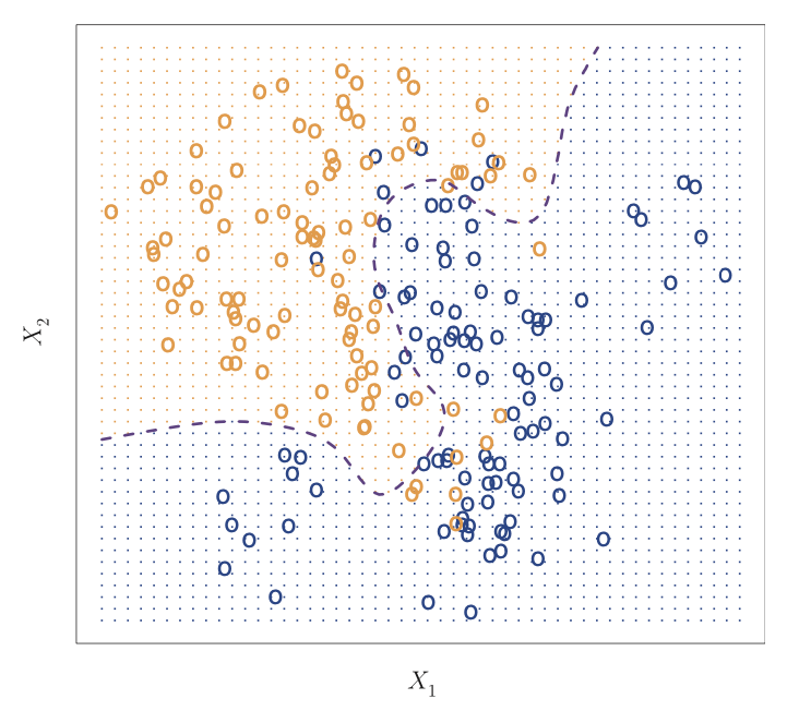
Source: An Introduction to Statistical Learning

A hundred observations are classified into two classes represented by orange and blue. The orange dots represent the area where a test observation will be assigned to the orange class while the blue dots represent the area where an observation will be assigned to the blue class. The dashed line is the Bayes Classifier.

K-Nearest Neighbor Classifier:

Unfortunately, the real decision boundary is rarely known in real world problems and the computing of the Bayes classifier is impossible.  One of the most frequently cited classifiers introduced that does a reasonable job instead is called K-Nearest Neighbors (KNN) Classifier.

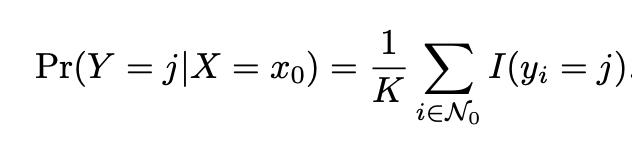
As with many other classifiers, the KNN classifier estimates the conditional distribution of Y given X and then classifies the observation to the class with the highest estimated probability.

Provided a positive integer K and a test observation of ,  the classifier identifies the K points in the data that are closest to x₀. Therefore if K is 5, then the five closest observations to observation x₀ are identified. These points are typically represented by N₀. The KNN classifier then computes the conditional probability for class j as the fraction of points in observations in N₀ whose response equals j.  The mathematical representation of this is: 

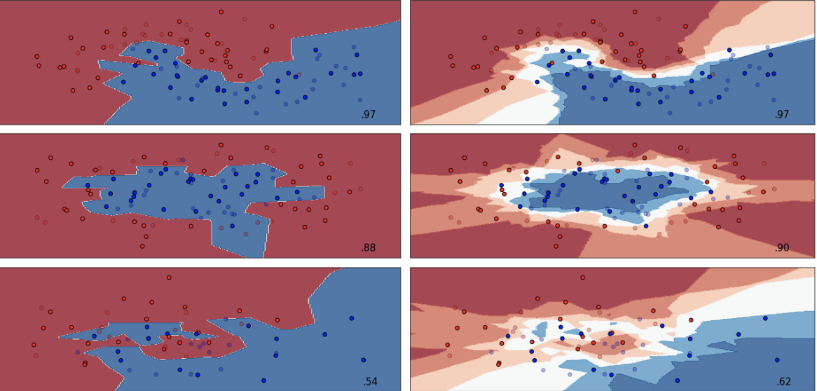
It is not surprising that altering K produces dramatically different results.  When K=1, the decision boundary is minimally restricted,  KNN models are said to produce low bias but high variance.  As we increase K, the flexibility of the classifier gets reduced and the decision boundary gets closer and closer to linear. These models produce low variance but high bias.  Neither perform particularly well based on test accuracy so we need to find a model with well balanced variance and bias, and we can find that model through parameter tuning. 

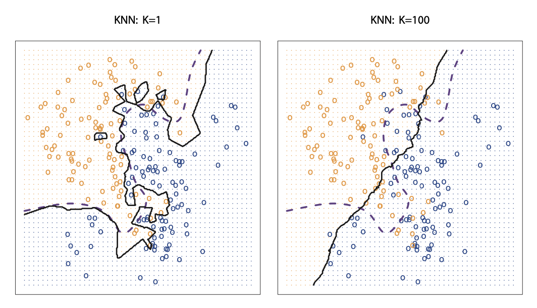
Source: An Introduction to Statistical Learning

The visual shows the difference between the KNN decision boundaries when K=1 vs. when K=100. It is clear that as K gets larger, the decision boundary resembles a liner line.

Use Python to fit KNN MODEL:

So let us tune a KNN model with GridSearchCV. The first step is to load all libraries and the charity data for classification. Note that I created three separate datasets: 1.) the original data set wit 21 variables that were partitioned into train and test sets, 2.) a dataset that contains second order polynomials and interaction terms also partitioned, and 3.) a a dataset that contains third order polynomials and interaction terms - partitioned into train and test sets. Each dataset was standardized and the variables with VIF scores greater than 5 were removed. All datasets were pickled and those pickles are called and loaded below. The pre-work described above can be seen by navigating to the Linear and Quadratic Discriminant Analysis blog.

import pandas as pd
import sklearn
import numpy as np
import matplotlib.pyplot as plt
from matplotlib.colors import ListedColormap

from sklearn.model_selection import train_test_split
from sklearn.neighbors import KNeighborsClassifier
from sklearn.neighbors import RadiusNeighborsClassifier

from sklearn.model_selection import GridSearchCV

from sklearn import metrics 
from sklearn.metrics import confusion_matrix
from sklearn.metrics import classification_report
from sklearn.metrics import roc_auc_score

from sklearn.preprocessing import StandardScaler

#read csv file
charity_df = pd.read_csv('charity.csv')

charity_df = pd.read_csv('charity.csv') #read csv file
charity_df=charity_df.dropna() #remove all lines with missing observations
charity_df = charity_df.drop('damt', axis=1) #drop damt

#Create regressors and dependent variable
X = charity_df.drop(['donr', 'ID'], axis=1) #note that donr was dropped from X because it is the dependent variable
y = charity_df['donr']

#Create training and test datasets
X_train, X_test, y_train, y_test = sklearn.model_selection.train_test_split(X, y, test_size = 0.20, random_state = 5)

import pickle
##### Get pickled files
# The original of the pickle is from the LDA/QDA file

X_test=pd.read_pickle('X_test.pkl') #read pickle
X_train=pd.read_pickle('X_train.pkl')
X_test_2=pd.read_pickle('X_test_2.pkl')
X_train_2=pd.read_pickle('X_train_2.pkl')
X_test_3=pd.read_pickle('X_test_3.pkl')
X_train_3=pd.read_pickle('X_train_3.pkl')

The untuned KNN model can serve as a baseline model in terms of test accuracy. The basic code structure looks like this:

#Default KNN model without any tuning - base metric
KNN_model_default = KNeighborsClassifier()
KNN_model_default.fit(X_train, y_train)
y_pred_KNN_default =KNN_model_default.predict(X_test)

We use cross validation and grid search to find the best model. Scikit-Learn affords us with several tunable parameters. For a complete list of tunable parameters click on the link for KNeighborsClassifier.
The list of tunable parameters are is also embedded (and coded out) in the chunk below. Further, I set the algorithm used to auto, although there are other parameters levels that one can decide on. Note that there are four options for algorithm:

• ball_tree’ will use BallTree

• ‘kd_tree’ will use KDTree

• ‘brute’ will use a brute-force search

• auto

At some point I tried these options but even then I removed brute from the list because the leaf size cannot be specified with that option.

#Parameter tuning with GridSearchCV 

#######################
### K-Nearest Neighbors
#######################
estimator_KNN = KNeighborsClassifier(algorithm='auto')
parameters_KNN = {
    'n_neighbors': (1,10, 1),
    'leaf_size': (20,40,1),
    'p': (1,2),
    'weights': ('uniform', 'distance'),
    'metric': ('minkowski', 'chebyshev'),
                   
# with GridSearch
grid_search_KNN = GridSearchCV(
    estimator=estimator_KNN,
    param_grid=parameters_KNN,
    scoring = 'accuracy',
    n_jobs = -1,
    cv = 5
)
#Documentation of tuneable parameters:
#class sklearn.neighbors.KNeighborsClassifier(n_neighbors=5, weights='uniform', 
#                                             algorithm='auto', leaf_size=30, p=2, 
#                                             metric='minkowski', metric_params=None, 
#                                             n_jobs=None, **kwargs)

The next step is to fit several models with the different datasets. Remember we have three different ones with first, second and third degree polynomials and interaction terms.

We can print several attributes based on GridSearchCV, one of which is the list of parameters for the best model:

• The leaf size was 20

• The distance metric used for the tree was Minkowski

• The umber of neighbors used for k neighbor queries was 10

• The power parameter for the Minkowski metric was 1 (When p = 1, this is equivalent to using manhattan_distance )

• All points in each neighborhood were weighted equally

KNN_1=grid_search_KNN.fit(X_train, y_train)
y_pred_KNN1 =KNN_1.predict(X_test)
KNN_2=grid_search_KNN.fit(X_train_2, y_train)
y_pred_KNN2 =KNN_2.predict(X_test_2)
KNN_3=grid_search_KNN.fit(X_train_3, y_train)
y_pred_KNN3 =KNN_3.predict(X_test_3)

#Parameter setting that gave the best results on the hold out data.
print(grid_search_KNN.best_params_ ) 
#Mean cross-validated score of the best_estimator
print('Best Score - KNN:', grid_search_KNN.best_score_ )

{'leaf_size': 20, 'metric': 'minkowski', 'n_neighbors': 10, 'p': 1, 'weights': 'uniform'}
Best Score - KNN: 0.8352426577796292

KNeighborsClassifier(algorithm='ball_tree', leaf_size=1, metric='minkowski',
                     metric_params=None, n_jobs=None, n_neighbors=150, p=2,
                     weights='distance')
{'algorithm': 'ball_tree', 'leaf_size': 1, 'n_neighbors': 150, 'weights': 'distance'}
0.5900853988752344

Now we can see how accurate teach of the four models performed based on test data. The first model was our default model without any tuning. Indeed, tuning parameters can get us significant gains over the accuracy of our default model. In fact, the model fitted on the original training data without interaction terms performed will and had an 86% accuracy.

print('Accuracy Score - KNN - Default:', metrics.accuracy_score(y_test, y_pred_KNN_default))  
print('Accuracy Score - KNN - Poly = 1:', metrics.accuracy_score(y_test, y_pred_KNN1)) 
print('Accuracy Score - KNN - Poly = 2:', metrics.accuracy_score(y_test, y_pred_KNN2)) 
print('Accuracy Score - KNN - Poly = 3:', metrics.accuracy_score(y_test, y_pred_KNN3)) 

Accuracy Score - KNN - Default: 0.8251457119067444
Accuracy Score - KNN - Poly = 1: 0.861781848459617
Accuracy Score - KNN - Poly = 2: 0.835970024979184
Accuracy Score - KNN - Poly = 3: 0.8343047460449625

Additional statistics are also available about the accuracy of the winning model. Take a look at the recall of our winning model for example. It will be really interesting to compare these results to the output of other methods.

print('BEST K-NEAREST NEIGHBORS MODEL')
print('Accuracy Score - KNN:', metrics.accuracy_score(y_test, y_pred_KNN1))  
print('Average Precision - KNN:', metrics.average_precision_score(y_test, y_pred_KNN1)) 
print('F1 Score - KNN:', metrics.f1_score(y_test, y_pred_KNN1)) 
print('Precision - KNN:', metrics.precision_score(y_test, y_pred_KNN1)) 
print('Recall - KNN:', metrics.recall_score(y_test, y_pred_KNN1))
print('ROC Score - KNN:', roc_auc_score(y_test, y_pred_KNN1))

#BEST K-NEAREST NEIGHBORS MODEL
Accuracy Score - KNN: 0.861781848459617
Average Precision - KNN: 0.7910641844215937
F1 Score - KNN: 0.8742424242424243
Precision - KNN: 0.8036211699164345
Recall - KNN: 0.9584717607973422
ROC Score - KNN: 0.8615397201315594