

Multi-layer Perceptron

““It is literally the case that learning makes you smarter.””
Revised Feb. 16, 2020
TABLE OF CONTENTS:
In order to arrive at the most accurate prediction, machine learning models are built, tuned and compared against each other. The reader can get can click on the links below to assess the models or sections of the exercise. Each section has a short explanation of theory, and a description of applied machine learning with Python:
Multi-Layer Perceptron (Current Blog)
OBJECTIVES:
This blog is part of a series of models showcasing applied machine learning models in a classification setting. By clicking on any of the tabs above, the reader can navigate to other methods of analysis applied to the same data. This was designed so that one could see what a data scientist would do from soup to nuts when faced with a problem like the one presented here. Note that the overall focus of this blog is Artificial Neural Networks. More specifically,
Understand the basics of Artificial Neural Networks;
Know that several ANNs exist;
Learn about how to fit and evaluate Multi-layer Perceptron; and
Use machine learning to tune a Multi-layer Perceptron model.
What are Artificial Neural Networks?
Artificial neural networks mimic the neuronal makeup of the brain. These networks represent the complex sets of switches that transmit electric or chemical impulses. In fact the network is so complex that each neuron may be connected to thousands of other neurons, and these connections are then repeatedly activated. Repeated activation results in learning.
So how do we train an artificial neural network to recognize and distinguish two classes? The answer is repetition. We repeatedly pass data through the ANN and pass back information about the learning performance. The repeated learning and feedback results in true system learning, much like the brain.
Neural networks do have some typical components: (a) an input layer, (b) hidden layers (their number can range from 0 to a lot), (c) an output layer, (d) weights and biases, and (e) an activation function.
Activation Function:
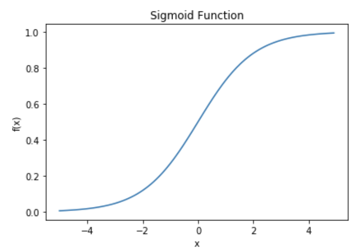
In an artificial neural network there is an activation function that serves the same task as the neuron does in the brain. This activation function is usually a sigmoid function used for classification similar to how the sigmoid function is used for classification in logistic regression. The sigmoid function moves from 0 to 1 as x reaches and surpasses a certain value (in this case 0). Of course other functions are also available. In fact, Scikit-Learn allows the tuning of a feed forward neural network called MLPerceptron (More on that later), and it offers four different activation functions when doing so:
‘identity’, no-op activation, useful to implement linear bottleneck, returns f(x) = x
‘Our current favorite: logistic’, the logistic sigmoid function, returns f(x) = 1 / (1 + exp(-x)). This is the sigmoid function discussed below.
‘tanh’, the hyperbolic tan function, returns f(x) = tanh(x).
‘relu’, the rectified linear unit function, returns f(x) = max(0, x)
import matplotlib.pyplot as plt
import numpy as np
import math

def sigmoid(x):
    a = []
    for item in x:
        a.append(1/(1+math.exp(-item)))
    return a
x = np.arange(-5., 5., 0.1)
sig = sigmoid(x)
plt.plot(x,sig)
plt.xlabel('x')
plt.ylabel('f(x)')
plt.title('Sigmoid Function')
plt.show()
Perceptron:
The activation functions (or neurons in the brain) are connected with each other through layers of nodes. Nodes are connected with each other so that the output of one node is an input of another. The inputs a node gets are weighted, which then are summed and the activation function is applied to them. The weighted sums of inputs applied to the activation function will then become an output. Take a look at the definition of a PERCEPTRON below.
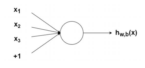
Perceptron
A NODE WITH INPUTS: The circle is a node, which houses he activation function. The node takes weighted inputs, sums them, then inputs them to the activation function.
Source: Adventures in Machine Learning
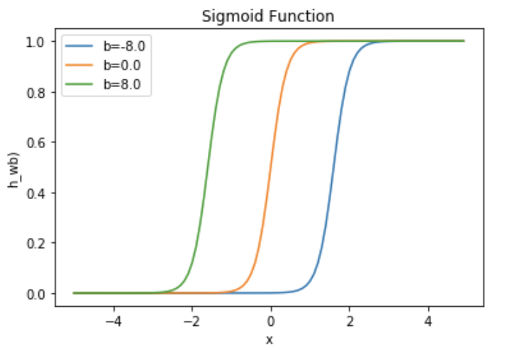
Bias:
Bias will change the sigmoid function in terms of when it will turn on vis-a-vis the value of x. The example below shows that the activation function gets activated (e.g. turns to 1) at a different value of x, which is caused by bias.
In the Perceptron and Bias sections we talked about weights and bias. These two constructs determine the strength of a predictive model in many models. In fact, computing predicted values is called feedforward, while updating weights and biases is called backpropagation. Backpropagation uses gradient descent to arrive at better updated weights and biases.
w=5.0
b1=-8.0
b2=0.0
b3=8.0
l1='b=-8.0'
l2='b=0.0'
l3='b=8.0'
for b, l in [(b1,l1),(b2,l2),(b3,l3)]:
    f=1/(1+np.exp(-(x*w+b)))
    plt.plot(x,f,label=l)
plt.xlabel('x')
plt.ylabel('h_wb)')
plt.legend(loc=2)
plt.title('Sigmoid Function')
plt.show()
Layers:
In neural networks, nodes can be connected a myriad of different ways. The most basic connectedness is an input layer, hidden layer and output layer. Layer 1 on the image below is the input layer, while layer 2 is a hidden layer. It is considered hidden because it is neither input nor output. Finally, layer 3 is the output layer.

Source: Adventures in Machine Learning
The structure of the layers determines the type of artificial neural network. The Asimov Institute published a really nice visual depicting a good cross-section of neural networks. The original article can be found at The Neural Network Zoo.

Multi-layer Perceptron:
In the next section, I will be focusing on multi-layer perceptron (MLP), which is available from Scikit-Learn. For other neural networks, other libraries/platforms are needed such as Keras.
MLP is a relatively simple form of neural network because the information travels in one direction only. It enters through the input nodes and exits through output nodes. This is referred as front propagation only. Interestingly, backpropagation is a training algorithm where you feed forward the values, calculate the error and propagate it back to the earlier layers. In other words, forward-propagation is part of the backpropagation algorithm but comes before back-propagating the signals from the nodes.
Also, the network may not even have to have a hidden layer. As a result, MLP belongs to a group of artificial neural networks called feed forward neural networks.
Predict Donations with Python:
As usual, load all required libraries and ingest data for analysis. The first step is to load all libraries and the charity data for classification. Note that I created three separate datasets: 1.) the original data set wit 21 variables that were partitioned into train and test sets, 2.) a dataset that contains second order polynomials and interaction terms also partitioned, and 3.) a a dataset that contains third order polynomials and interaction terms - partitioned into train and test sets. Each dataset was standardized and the variables with VIF scores greater than 5 were removed. All datasets were pickled and those pickles are called and loaded below. The pre-work described above can be seen by navigating to the Linear and Quadratic Discriminant Analysis blog.
import pandas as pd
import sklearn
import numpy as np

from sklearn.model_selection import train_test_split
from sklearn.neural_network import MLPClassifier

from sklearn import metrics
from sklearn import neural_network
from sklearn.metrics import confusion_matrix
from sklearn.metrics import classification_report

from sklearn.model_selection import GridSearchCV
from sklearn.metrics import roc_auc_score

#read csv file
charity_df = pd.read_csv('charity.csv')

charity_df = pd.read_csv('charity.csv') #read csv file
charity_df=charity_df.dropna() #remove all lines with missing observations
charity_df = charity_df.drop('damt', axis=1) #drop damt

#Create regressors and dependent variable
X = charity_df.drop(['donr', 'ID'], axis=1) #note that donr was dropped from X because it is the dependent variable
y = charity_df['donr']

#Create training and test datasets
X_train, X_test, y_train, y_test = sklearn.model_selection.train_test_split(X, y, test_size = 0.20, random_state = 5)

import pickle
##### Get pickled files
# The original of the pickle is from the LDA/QDA file

X_test=pd.read_pickle('X_test.pkl') #read pickle
X_train=pd.read_pickle('X_train.pkl')
X_test_2=pd.read_pickle('X_test_2.pkl')
X_train_2=pd.read_pickle('X_train_2.pkl')
X_test_3=pd.read_pickle('X_test_3.pkl')
X_train_3=pd.read_pickle('X_train_3.pkl')
The first model we’ll fit will be untuned and will serve as a baseline to compare to when assessing the the accuracy of tuned models.
#Default Neural Network model without any tuning - base metric
MLP_model_default = MLPClassifier()
MLP_model_default.fit(X_train, y_train)
y_pred_MLP_default =MLP_model_default.predict(X_test)
Multi-layer Perceptron allows the automatic tuning of parameters. We will tune these using GridSearchCV(). A list of tunable parameters can be found at the MLP Classifier Page of Scikit-Learn. One of the issues that one needs to pay attention to is that the choice of a solver influences which parameter can be tuned. As a result, I split up the task into three tasks with three different solvers.
#Parameter tuning with GridSearchCV

#######################
### Neural Network
#######################
estimator_MLP = MLPClassifier(batch_size='auto', warm_start=True, max_iter=400)
parameters_MLP = {
    'hidden_layer_sizes': (10,120,10),
    'activation': ('identity', 'logistic', 'tanh', 'relu'),
    'alpha': (0.000001, 0.00001, 0.0001),
    'solver': ('lbfgs', 'sgd', 'adam'),
    'shrinking': (True, False),
                   }
# with GridSearch
grid_search_MLP = GridSearchCV(
    estimator=estimator_MLP,
    param_grid=parameters_MLP,
    scoring = 'accuracy',
    n_jobs = -1,
    cv = 5
)
#######################
### Neural Network (Solver=sgd)
#######################

estimator_MLP_B = MLPClassifier(batch_size='auto', warm_start=True, solver='sgd', max_iter=400, early_stopping=True)
parameters_MLP_B = {
    'hidden_layer_sizes': (10,120,10),
    'activation': ('identity', 'logistic', 'tanh', 'relu'),
    'alpha': (0.000001, 0.00001, 0.0001),
    'learning_rate': ('constant', 'invscaling', 'adaptive'),
    'momentum': (0.1,0.9,0.1),
                   }
# with GridSearch
grid_search_MLP_B = GridSearchCV(
    estimator=estimator_MLP_B,
    param_grid=parameters_MLP_B,
    scoring = 'accuracy',
    n_jobs = -1,
    cv = 5
)
#######################
### Neural Network (Solver=adam)
#######################
estimator_MLP_C = MLPClassifier(batch_size='auto', warm_start=True, solver='adam', max_iter=400, early_stopping=True)
parameters_MLP_C = {
    'hidden_layer_sizes': (10,120,10),
    'activation': ('identity', 'logistic', 'tanh', 'relu'),
    'alpha': (0.000001, 0.00001, 0.0001),
    'beta_1': (0.1,0.9,0.1),
    'beta_2': (0.1,0.9,0.1),
                   }
# with GridSearch
grid_search_MLP_C = GridSearchCV(
    estimator=estimator_MLP_C,
    param_grid=parameters_MLP_C,
    scoring = 'accuracy',
    n_jobs = -1,
    cv = 5
)

#Documentation of tuneable parameters:
#class sklearn.neural_network.MLPClassifier(hidden_layer_sizes=(100, ),
#                                           activation='relu', solver='adam', alpha=0.0001, batch_size='auto',
#                                           learning_rate='constant', learning_rate_init=0.001, power_t=0.5,
#                                           max_iter=200, shuffle=True, random_state=None, tol=0.0001, verbose=False,
#                                           warm_start=False, momentum=0.9, nesterovs_momentum=True,
#                                           early_stopping=False, validation_fraction=0.1, beta_1=0.9, beta_2=0.999,
#                                           epsilon=1e-08, n_iter_no_change=10, max_fun=15000)
We now fit several models: there are three datasets (1st, 2nd and 3rd degree polynomials) to try and three different solver options (the first grid has three options and we are asking GridSearchCV to pick the best option, while in the second and third grids we are specifying the sgd and adam solvers, respectively) to iterate with:
MLP_1=grid_search_MLP.fit(X_train, y_train)
y_pred_MLP1 =MLP_1.predict(X_test)
MLP_1_B=grid_search_MLP_B.fit(X_train, y_train)
y_pred_MLP1_B =MLP_1_B.predict(X_test)
MLP_1_C=grid_search_MLP_C.fit(X_train, y_train)
y_pred_MLP1_C =MLP_1_C.predict(X_test)

MLP_2=grid_search_MLP.fit(X_train_2, y_train)
y_pred_MLP2 =MLP_2.predict(X_test_2)
MLP_2_B=grid_search_MLP_B.fit(X_train_2, y_train)
y_pred_MLP2_B =MLP_2_B.predict(X_test_2)
MLP_2_C=grid_search_MLP_C.fit(X_train_2, y_train)
y_pred_MLP2_C =MLP_2_C.predict(X_test_2)

MLP_3=grid_search_MLP.fit(X_train_3, y_train)
y_pred_MLP3 =MLP_3.predict(X_test_3)
MLP_3_B=grid_search_MLP_B.fit(X_train_3, y_train)
y_pred_MLP3_B =MLP_3_B.predict(X_test_3)
MLP_3_C=grid_search_MLP_C.fit(X_train_3, y_train)
y_pred_MLP3_C =MLP_3_C.predict(X_test_3)
We can compute the accuracy associated with each of the models. The best model appears to be the one using the automatically selected solver based on the original training data. This model had a test accuracy of 90.6%.
print('Accuracy Score - Neural Net - Default:', metrics.accuracy_score(y_test, y_pred_MLP_default))
print('Accuracy Score - Neural Net - Poly = 1:', metrics.accuracy_score(y_test, y_pred_MLP1))
print('Accuracy Score - Neural Net - Poly = 2:', metrics.accuracy_score(y_test, y_pred_MLP2))
print('Accuracy Score - Neural Net - Poly = 3:', metrics.accuracy_score(y_test, y_pred_MLP3))
print('')
print('')
print('Accuracy Score - Neural Net (sgd) - Poly = 1:', metrics.accuracy_score(y_test, y_pred_MLP1_B))
print('Accuracy Score - Neural Net (sgd) - Poly = 2:', metrics.accuracy_score(y_test, y_pred_MLP2_B))
print('Accuracy Score - Neural Net (sgd) - Poly = 3:', metrics.accuracy_score(y_test, y_pred_MLP3_B))
print('')
print('')
print('Accuracy Score - Neural Net (adam) - Poly = 1:', metrics.accuracy_score(y_test, y_pred_MLP1_C))
print('Accuracy Score - Neural Net (adam) - Poly = 2:', metrics.accuracy_score(y_test, y_pred_MLP2_C))
print('Accuracy Score - Neural Net (adam) - Poly = 3:', metrics.accuracy_score(y_test, y_pred_MLP3_C))

Accuracy Score - Neural Net - Default: 0.9050791007493755
Accuracy Score - Neural Net - Poly = 1: 0.9059117402164862
Accuracy Score - Neural Net - Poly = 2: 0.8784346378018318
Accuracy Score - Neural Net - Poly = 3: 0.858451290591174


Accuracy Score - Neural Net (sgd) - Poly = 1: 0.8376353039134055
Accuracy Score - Neural Net (sgd) - Poly = 2: 0.884263114071607
Accuracy Score - Neural Net (sgd) - Poly = 3: 0.8209825145711906


Accuracy Score - Neural Net (adam) - Poly = 1: 0.9017485428809325
Accuracy Score - Neural Net (adam) - Poly = 2: 0.8900915903413822
Accuracy Score - Neural Net (adam) - Poly = 3: 0.8467943380516236
Let us compute some additional accuracy statistics for the winning models for the three grid searches. A very interesting dilemma appears, since the recall of the model using the adam solver appears to be better:
print('BEST Multi-layer Perceptron classifier')
print('Accuracy Score - Neural Net:', metrics.accuracy_score(y_test, y_pred_MLP1))
print('Average Precision - Neural Net:', metrics.average_precision_score(y_test, y_pred_MLP1))
print('F1 Score - Neural Net:', metrics.f1_score(y_test, y_pred_MLP1))
print('Precision - Neural Net:', metrics.precision_score(y_test, y_pred_MLP1))
print('Recall - Neural Net:', metrics.recall_score(y_test, y_pred_MLP1))
print('ROC Score - Neural Net:', roc_auc_score(y_test, y_pred_MLP1))
print('')
print('')


print('BEST Multi-layer Perceptron classifier (sgd solver)')
print('Accuracy Score - Neural Net:', metrics.accuracy_score(y_test, y_pred_MLP1_B))
print('Average Precision - Neural Net:', metrics.average_precision_score(y_test, y_pred_MLP1_B))
print('F1 Score - Neural Net:', metrics.f1_score(y_test, y_pred_MLP1_B))
print('Precision - Neural Net:', metrics.precision_score(y_test, y_pred_MLP1_B))
print('Recall - Neural Net:', metrics.recall_score(y_test, y_pred_MLP1_B))
print('ROC Score - Neural Net:', roc_auc_score(y_test, y_pred_MLP1_B))
print('')
print('')

print('BEST Multi-layer Perceptron classifier (adam solver)')
print('Accuracy Score - Neural Net:', metrics.accuracy_score(y_test, y_pred_MLP1_C))
print('Average Precision - Neural Net:', metrics.average_precision_score(y_test, y_pred_MLP1_C))
print('F1 Score - Neural Net:', metrics.f1_score(y_test, y_pred_MLP1_C))
print('Precision - Neural Net:', metrics.precision_score(y_test, y_pred_MLP1_C))
print('Recall - Neural Net:', metrics.recall_score(y_test, y_pred_MLP1_C))
print('ROC Score - Neural Net:', roc_auc_score(y_test, y_pred_MLP1_C))

BEST Multi-layer Perceptron classifier
Accuracy Score - Neural Net: 0.9059117402164862
Average Precision - Neural Net: 0.865705917350576
F1 Score - Neural Net: 0.9068425391591095
Precision - Neural Net: 0.900163666121113
Recall - Neural Net: 0.9136212624584718
ROC Score - Neural Net: 0.9058924342342443


BEST Multi-layer Perceptron classifier (sgd solver)
Accuracy Score - Neural Net: 0.8376353039134055
Average Precision - Neural Net: 0.7775204442317897
F1 Score - Neural Net: 0.8423605497170573
Precision - Neural Net: 0.8204724409448819
Recall - Neural Net: 0.8654485049833887
ROC Score - Neural Net: 0.837565654828923


BEST Multi-layer Perceptron classifier (adam solver)
Accuracy Score - Neural Net: 0.9017485428809325
Average Precision - Neural Net: 0.8580074958075786
F1 Score - Neural Net: 0.9034369885433715
Precision - Neural Net: 0.8903225806451613
Recall - Neural Net: 0.9169435215946844
ROC Score - Neural Net: 0.90171049201604

