
Model Selection

““All models are wrong, but some are useful.””
TABLE OF CONTENTS:
We have now fitted several models using machine learning and we are ready to compare the test accuracy of the final models. A list of all models can be found below. Each section has a short explanation of theory, and a description of applied machine learning with Python:
Model Comparisons
OBJECTIVES:
This blog is part of a series of models showcasing applied machine learning models in a classification setting. By clicking on any of the tabs above, the reader can navigate to other methods of analysis applied to the same data. This was designed so that one could see what a data scientist would do from soup to nuts when faced with a problem like the one presented here. The overall focus of this blog is model selection based on test accuracy.
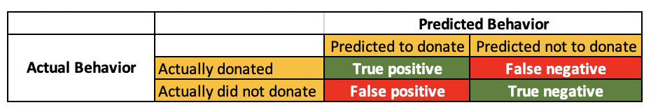
Confusion Matrix:
The command confusion_matrix creates an array, that shows the number of true positives (TP), false positives (FP), false negatives (FN) and true negatives (TN). These items can be used extensively for assessing the accuracy of any model.
With the data in hand, we can calculate several important statistics to assess the accuracy of our model. Here is a list of statistics of potential interest
sensitivity, recall, hit rate, or true positive rate (TPR): (TP / (TP + FN))
specificity, selectivity or true negative rate (TNR): (TN / (TN + FP))
precision or positive predictive value (PPV): (TP / (TP + FP))
negative predictive value (NPV): (TN / (TN + FN))
miss rate or false negative rate (FNR): (FN / (FN + TP))
fall-out or false positive rate (FPR): (FP / (FP + TN))
false discovery rate (FDR): (FP / (FP + TP))
false omission rate (FOR): (FN / (FN + TN))
threat score (TS) or Critical Success Index (CSI): (TP / (TP + FN + FP))
accuracy (ACC): (TP+TN) / (TP+FP+FN + TN))
F1: 2*TP/(2*TP+FP+FN)
ACCURACY, precision, recall, F1 score:
We want to pay special attention to accuracy, precision, recall, and the F1 score. Accuracy is a performance metric that is very intuitive: it is simply the ratio of all correctly predicted cases whether positive or negative and all cases in the data.
Precision is the ratio of correctly predicted positive cases vs. all predicted positive cases. It answers the following question: Of all people in the database we predicted as donors, how many were actually donors? If we think about it, high precision should yield to a low false positive rate. This is important if our budget for the direct mail campaign is limited, we want to limit sending mail in error to those who will not respond! If we want to maximize our profit, precision is key.
Recall or sensitivity is the ratio of all correctly identified positive cases divided by all actually positive cases. It answers the following question: How well did our model perform in correctly identifying donors among all true donors. This is important if we want to maximize overall response (call it revenue maximization), since we want to leave off as few actual donors from our campaign as possible!
The F1 Score is the weighted average of precision and recall, hence it takes both false positives and false negatives into account. If data has an uneven class distribution, then the F1 score is far more useful than accuracy. Accuracy works best if false positives and false negatives have similar cost. If the cost of false positives and false negatives are very different, it’s better to look at both precision and recall.
ROC AUC:
ROC stands for Receiver Operating Characteristic, which is a World War II term used to evaluate the performance of radar. We discussed specificity and sensitivity before, but to refresh: sensitivity is the proportion of correctly predicted events (cases), while specificity is the the proportion of correctly identified non-events (cases). Ideally, both specificity and sensitivity should be high. The ROC curve represents the tradeoff between the two constructs.
The ROC-AUC score provides us with information about how well a model is performing its job of separating cases: in our case distinguishing donors from those not donating. A 0.91 score means that there is a 91% chance that a model can distinguish donors from non-donors.
Results:
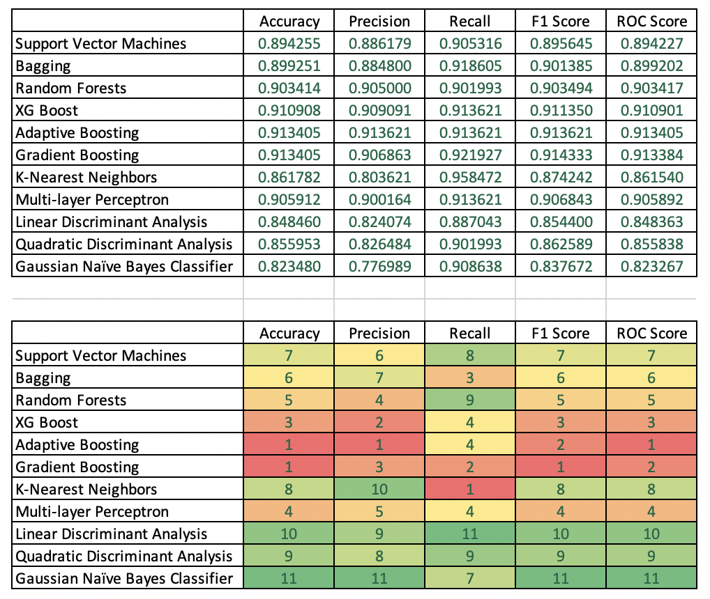
The table below lists accuracy statistics of the various model types. The second table ranks models column-wise, e.g. identifies the best models based on one of five accuracy metrics.
Accuracy: Adaptive Boosting and Gradient Boosting produced the best test accuracy with identical scores at 91.34.
Precision: Adaptive Boosting was a clear winner followed by XG Boost and and Gradient Boosting in second and third place, respectively.
Recall: K-Nearest Neighbors was the strongest by far with a score of 95.85. Gradient Boosting was second.
F1 Score: Gradient Boosting was best, followed by Adaptive Boosting and XG Boost, respectively.
ROC Score: Adaptive Boosting achieved the best score followed by gradient boosting and then XG Boost.

The verdict:
A not-for-profit organization is likely to be forced to use its marketing budget as judiciously as possible: Profitability is key. As a result, precision and the F1 score are most important. As a result, adaptive boosting therefore is probably a better choice as it provides the same accuracy as gradient boosting but with better precision. While gradient boosting has a better F1 score than that of adaptive boosting, the difference is minimal. Further, adaptive boosting has a better ROC score implying that that model is better at separating donors from non-donors.
