Support Vector Machines

““Before machines the only from of entertainment people really had was relationships.””
Revised Feb. 16, 2020
TABLE OF CONTENTS:
In order to arrive at the most accurate prediction, machine learning models are built, tuned and compared against each other. The reader can get can click on the links below to assess the models or sections of the exercise. Each section has a short explanation of theory, and a description of applied machine learning with Python:
Support Vector Machines (Current Blog)
OBJECTIVES:
This blog is part of a series of models showcasing applied machine learning models in a classification setting. By clicking on any of the tabs above, the reader can navigate to other methods of analysis applied to the same data. This was designed so that one could see what a data scientist would do from soup to nuts when faced with a problem like the one presented here. Note that the overall focus of this blog is Support Vector Machines. More specifically,
Learn about maximal margin and support vector classifier, hyperplanes and support vectors;
Understand kernels and support vector machines;
Observe the impact of various kernels on SVM output;
Study how to tune parameters in SVM using cross validation;
Find out what’s tunable in various SVM libraries; and
Practice patience: SVMs are notoriously slow to run!
Introduction:
Support Vector Machine (SVM) is a classification method frequently used in text analytics, handwriting and face recognition and other classification problems because it tends to produce very accurate results compared to competing methods in machine learning. Note that SVM can be used for regression as well, although the method is most frequently associated with classification problems.
SVM is a generalization of a classifier called maximal margin classifier. Unfortunately, when using a maximal margin classifier, classes need to be separated by a linear boundary, which is not practical in most cases. Since most classification problems require non-linear class boundaries, and observations are seldom cleanly classified without overlap, SVM offers an excellent solution by introducing the support vector classifier. But first, let’s establish what a few constructs actually mean.
Hyperplanes:
A hyperplane is a flat subspace in dimension p-1. In a two-dimensional space, the hyperplane is a simple line. In a three-dimensional space, it is a flat two-dimensional subspace. In higher dimensions, the hyperplane is always a flat p-1-dimensional subspace. The mathematical equation for a hyperplane is:

Let’s take the example of a two-dimensional hyperplane that is divided by:
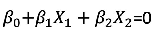
If X satisfies the condition, then it lies directly on the line. If X does not satisfy the condition, then it lies on one of two sides of the hyperplane depending on whether the first or the second condition is true:

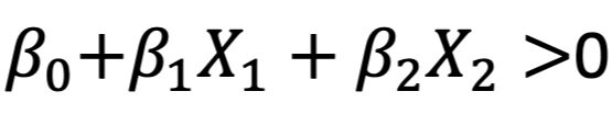
As a result, the hyperplane can be used as a classifier because in the above case, the two-dimensional space is divided into two sub-spaces by the hyperplane, which in this case is a line.
The Maximal Margin Classifier:
If data can be separated perfectly, then there is an infinite number of hyperplanes. The maximal margin hyperplane can be computed by finding the hyperplane that is farthest from the training observations. The perpendicular distance between each observation and all potential hyperplanes is measured. The largest distance between the observations and the hyperplane is known as the maximal margin, which can be used for classification of observations. Large distances should make us more comfortable that the differences between the two classes are real.

Source: Introduction to Statistical Learning (Click for link)
Margin is the gap between the two dashed lines. They were defined by calculating the perpendicular distance(s) from the hyperplane to support vectors (in this case, the closest points). A larger margin between two classes is preferred!
There are three training observations in this example that are at an equal distance from the maximal margin hyperplane and are depicted on the dashed lines. They represent the width of the margin and are called support vectors. If these points moved, the hyperplane would move as well. Interestingly, the movement of any other observation has no effect on the hyperplane.
Support Vector Classifiers:
It has been discussed earlier that when observations are not completely separable then a maximal margin classifier will not offer a solution. We may be OK with minimal misclassification of training data. At that point, a support vector classifier may be an appropriate choice.
Maximal margin classifiers require observations to be on the correct side of the hyperplane and margin. But what if we allowed some observations to be on the incorrect side of the margin or even hyperplane? Well, when using the support vector classifier, the hyperplane is not used for classification. At that point, using the support vector classifier is an optimization problem with the objective function targeting as few misclassified cases as possible. The mathematical depiction of the optimization problem is below.

Here, C is a tuning parameter to be tuned via cross validation an εi are slack variables that allow for misclassification. A small C means narrow margins resulting in low bias but high variance. A large C results in a wide margin, which means high bias but low variance.
Only observations directly on the margin or observations that violate the margin have an effect on the hyperplane. As a result, correctly classified observations have no effect on the support vector classifier. Consequently, the observations that lie directly on the margins or observations on the wrong side of the margin are called support vectors. When C is large, then more observations violate the margin, and there are more support vectors. When C is small, violating observations are fewer in number and there are few support vectors.
Support Vector Machines:
Support vector classifiers are great for two-class problems where the boundary between the classes is linear. Unfortunately, real life rarely produces linear boundaries. When the data is non-linear, we can introduce terms that are non-linear and then use support vector classifiers. The resulting problem is still an optimization issue.
SVM is an extension of the support vector classifier as a result of the increased feature space using kernels. A kernel is a function that measures the similarity between two observations. Kernels can be linear or polynomial (e.g. non-linear) When the non-linear kernel and support vector classifier are combined to form a classifier, the resulting classifier is known as the support vector machine. Here is an example of a SVM with a third degree polynomial kernel and a SVM with a radial kernel.

Use Python to fit SVM:
As usual, load all required libraries and ingest data for analysis. The first step is to load all libraries and the charity data for classification. Note that I created three separate datasets: 1.) the original data set wit 21 variables that were partitioned into train and test sets, 2.) a dataset that contains second order polynomials and interaction terms also partitioned, and 3.) a dataset that contains third order polynomials and interaction terms - partitioned into train and test sets. Each dataset was standardized and the variables with VIF scores greater than 5 were removed. All datasets were pickled and those pickles are called and loaded below. The pre-work described above can be seen by navigating to the Linear and Quadratic Discriminant Analysis blog.
import pandas as pd
import sklearn
import numpy as np

from sklearn.model_selection import train_test_split
from sklearn import svm
from sklearn.svm import SVC
from sklearn.svm import LinearSVC

from sklearn import metrics
from sklearn import neural_network
from sklearn.metrics import confusion_matrix
from sklearn.metrics import classification_report

from sklearn.model_selection import GridSearchCV
from sklearn.metrics import roc_auc_score

#read csv file
charity_df = pd.read_csv('charity.csv')

charity_df = pd.read_csv('charity.csv') #read csv file
charity_df=charity_df.dropna() #remove all lines with missing observations
charity_df = charity_df.drop('damt', axis=1) #drop damt

#Create regressors and dependent variable
X = charity_df.drop(['donr', 'ID'], axis=1) #note that donr was dropped from X because it is the dependent variable
y = charity_df['donr']

#Create training and test datasets
X_train, X_test, y_train, y_test = sklearn.model_selection.train_test_split(X, y, test_size = 0.20, random_state = 5)

import pickle
##### Get pickled files
# The original of the pickle is from the LDA/QDA file

X_test=pd.read_pickle('X_test.pkl') #read pickle
X_train=pd.read_pickle('X_train.pkl')
X_test_2=pd.read_pickle('X_test_2.pkl')
X_train_2=pd.read_pickle('X_train_2.pkl')
X_test_3=pd.read_pickle('X_test_3.pkl')
X_train_3=pd.read_pickle('X_train_3.pkl')
Several versions of SVM are available in Scikit-learn. The firs to explore is sklearn.svm.SVC() . We will also use this as a baseline model when assessing the test accuracy of tuned models as this model is not yet tuned.
#Default SVM model without any tuning - base metric
SVC_model_default = SVC()
SVC_model_default.fit(X_train, y_train)
y_pred_SVC_default =SVC_model_default.predict(X_test)
Since our goal is to find the most accurate model possible based on test data, we will used GridSearchCV to tune the parameters of the model. A complete list of tunable parameters can be found by navigating to the SVM page operated by Scikit-Learn.
#Parameter tuning with GridSearchCV

#######################
### Support Vector Machines
#######################

estimator_SVM = SVC(gamma='scale')
parameters_SVM = {
    'C': (0.1, 15.0, 0.1),
    'kernel': ('linear', 'poly', 'rbf', 'sigmoid'),
    'coef0': (0.0, 10.0, 1.0),
    'shrinking': (True, False),

                   }

# with GridSearch
grid_search_SVM = GridSearchCV(
    estimator=estimator_SVM,
    param_grid=parameters_SVM,
    scoring = 'accuracy',
    n_jobs = -1,
    cv = 5
)
#class sklearn.svm.SVC(C=1.0, kernel='rbf', degree=3,
#                      gamma='scale', coef0=0.0, shrinking=True, probability=False, tol=0.001, cache_size=200,
#                      class_weight=None, verbose=False, max_iter=-1, decision_function_shape='ovr',
# .                    break_ties=False, random_state=None)
Fitting models with the three datasets discussed earlier is relatively easy. We can also print the attributes of models, one of which is the parameter list of the wining model.
SVM_1=grid_search_SVM.fit(X_train, y_train)
y_pred_SVM1 =SVM_1.predict(X_test)
SVM_2=grid_search_SVM.fit(X_train_2, y_train)
y_pred_SVM2 =SVM_2.predict(X_test_2)
SVM_3=grid_search_SVM.fit(X_train_3, y_train)
y_pred_SVM3 =SVM_3.predict(X_test_3)

#Parameter setting that gave the best results on the hold out data.
print(grid_search_SVM.best_params_)

{'C': 15.0, 'coef0': 0.0, 'kernel': 'rbf', 'shrinking': True}
The accuracy scores of each variable can be computed and printed for comparison. Also, several accuracy metrics of the winning model can be seen below, all of which need to be scrutinized when choosing a champion model for production.
print('Accuracy Score - SVM - Default:', metrics.accuracy_score(y_test, y_pred_SVC_default))
print('Accuracy Score - SVM - Poly = 1:', metrics.accuracy_score(y_test, y_pred_SVM1))
print('Accuracy Score - SVM - Poly = 2:', metrics.accuracy_score(y_test, y_pred_SVM2))
print('Accuracy Score - SVM - Poly = 3:', metrics.accuracy_score(y_test, y_pred_SVM3))
print('')

Accuracy Score - SVM - Default: 0.8884263114071607
Accuracy Score - SVM - Poly = 1: 0.8942547876769359
Accuracy Score - SVM - Poly = 2: 0.8800999167360533
Accuracy Score - SVM - Poly = 3: 0.858451290591174

print('BEST SVM')
print('Accuracy Score - SVM:', metrics.accuracy_score(y_test, y_pred_SVM1))
print('Average Precision - SVM:', metrics.average_precision_score(y_test, y_pred_SVM1))
print('F1 Score - SVM:', metrics.f1_score(y_test, y_pred_SVM1))
print('Precision - SVM:', metrics.precision_score(y_test, y_pred_SVM1))
print('Recall - SVM:', metrics.recall_score(y_test, y_pred_SVM1))
print('ROC Score - SVM:', roc_auc_score(y_test, y_pred_SVM1))

#BEST SVM
Accuracy Score - SVM: 0.8942547876769359
Average Precision - SVM: 0.8497320105469016
F1 Score - SVM: 0.8956450287592441
Precision - SVM: 0.8861788617886179
Recall - SVM: 0.9053156146179402
ROC Score - SVM: 0.894227089445865
Finally, SciKit-Learn offers other SVM libraries with the option to tune other parameters. The tunable parameter list as well as a list of attributes is available by clicking on the library names below:
Since most of what I wrote about so far was using sklearn.svm.SVC, I wanted to quickly show how LinearSVC works, since in this model the penalty type and loss function can be specified. We can observe the change in the loss function and its significant impact on model accuracy.
#Penalized svm
model_l2_sh = LinearSVC(penalty='l2', loss='squared_hinge', dual=True, tol=0.0001, C=3.0, multi_class='ovr', fit_intercept=True, intercept_scaling=1, class_weight=None, verbose=0, random_state=None, max_iter=1000)
model_l2_h = LinearSVC(penalty='l2', loss='hinge', dual=True, tol=0.0001, C=3.0, multi_class='ovr', fit_intercept=True, intercept_scaling=1, class_weight=None, verbose=0, random_state=None, max_iter=1000)

model_l2_sh.fit(X_train, y_train)
model_l2_h.fit(X_train, y_train)

y_pred_l2_sh =model_l2_sh.predict(X_test)
y_pred_l2_h =model_l2_h.predict(X_test)

print('Accuracy Score - l2 penalty- sq hinge loss:', metrics.accuracy_score(y_test, y_pred_l2_sh))
print('Accuracy Score - l2 penalty- hinge loss:', metrics.accuracy_score(y_test, y_pred_l2_h))

Accuracy Score - l2 penalty- sq hinge loss: 0.8351373855120733
Accuracy Score - l2 penalty- hinge loss: 0.5237302248126561