Ensemble Learning
““I can imagine wanting to work with this ensemble and this company always.””
TABLE OF CONTENTS:
In order to arrive at the most accurate prediction, machine learning models are built, tuned and compared against each other. The reader can get can click on the links below to assess the models or sections of the exercise. Each section has a short explanation of theory, and a description of applied machine learning with Python:
Ensemble Learning (Current Blog)
OBJECTIVES:
This blog is part of a series of models showcasing applied machine learning models in a classification setting. By clicking on any of the tabs above, the reader can navigate to other methods of analysis applied to the same data. This was designed so that one could see what a data scientist would do from soup to nuts when faced with a problem like the one presented here. Note that the overall focus of this blog is Ensemble Learning.
Classification Trees:
Before getting too deep in the forest (Ha!), I wanted to spend a few minutes on classification trees. They are similar to regression trees but have a qualitative response. At the end of 2019, I wrote about regression trees and pointed out that the predicted response for an observation is actually the mean of all training observations on the same terminal node. (Click here to navigate to the blog.) . In a classification problem, the predicted class that an observation belongs to is the most frequently occurring class in a terminal node based on training data.
The similarities do not end here. Growing trees in a classification setting is also similar to growing trees for regression. Recursive binary splitting is used for growing a tree, but the criterion to use for binary splits is classification error rate (instead of RSS for regression). That classification error rate is the fraction of training observations that do not belong to the most common class. In practice, two other measures are used, the Gini Index and entropy, both of which can be tried when tuning models with Scikit-Learn.
Ensemble Learning:
Similar to regression, individual classification trees can be grouped and tuned as ensemble models. When using ensemble methods multiple trees are being cultivated at the same time. Individual trees have high variance but low bias on an individual basis. When averaging the individual trees’ predicted values, the variance of the ensemble system is usually greatly reduced. In this blog the following ensemble models for classification will be discussed:
bagging
various boosting techniques
random forests
BAGGING:
The bootstrap approach can be used to dramatically improve the performance of decision trees. Decision trees often suffer from relatively high variance, which results in poor accuracy measured on the test data. Bootstrap aggregation or bagging means that repeated samples are taken from a single training dataset with replacement. Classification trees are separately fitted on each, and each model is used for predictions. These predictions are then averaged.
BOOSTING:
Boosting is also an ensemble method that can be used on a regression and classification setting. During boosting a sequence of trees is grown and successive trees are cultivated on the residuals of preceding trees. Note that during boosting, residuals are used, not the dependent variable for sequential tree fitting. When boosting, bootstrapping is not used but each tree is fit on the original data set. When the next sequence of trees is built, the residuals are updated. Boosting uses three main tuning parameters: the number of trees, a shrinkage parameter and the number of splits per tree. Cross-validation should be used to decide on the number of trees. The shrinkage parameter is usually a small number (0.01 or 0.001), and must be evaluated in the context of the number of trees used because a very small shrinkage parameter typically requires a large number of trees. The number of splits in each tree is used to control the complexity of the ensemble model. It is often sufficient to create a tree stump by setting this parameter to one.
Several versions of boosting are available for ensemble learning: (a) Adaptive Boosting, (b) Gradient Boosting, (c) Extreme Gradient Boosting, and (d) Light GBM.
RANDOM FORESTS:
Similar to bagging, random forests also make use of building multiple classification trees based on bootstrapped training samples. However, for each split in a tree, a random set of predictors is chosen from the full set of predictors. The size of the random subset is typically the square root of the total number of features. The split is allowed to choose only from the randomly selected subset of predictors. A fresh sample of predictors is taken at each split, which means that the majority of predictors are not allowed to be considered at each split. As a result, this process makes the individual trees less correlated.
Charity Analysis:
First, load all required libraries and data. Note that I partitioned the data, then standardized it and removed all collinear items based on VIF scores. The python code for this work can be found on the one of the prior blogs. Please click Linear and Quadratic Discriminant Analysis to see it.
import numpy as np
import pandas as pd
import matplotlib.pyplot as plt

import sklearn
from sklearn.preprocessing import PolynomialFeatures
from sklearn.preprocessing import StandardScaler

from sklearn.model_selection import train_test_split
from sklearn.model_selection import GridSearchCV
from sklearn import metrics
from sklearn.metrics import confusion_matrix
from sklearn.metrics import classification_report
from sklearn.metrics import roc_auc_score

import warnings

from sklearn.ensemble import RandomForestClassifier
from sklearn.ensemble import GradientBoostingClassifier
from sklearn.ensemble import AdaBoostClassifier
from sklearn.ensemble import BaggingClassifier
from sklearn.tree import DecisionTreeClassifier
from xgboost import XGBClassifier
I saved the treated datasets as pickles because some of the steps were very time consuming. Here, we just need to read the pickles. The first two is the original test and train dataset, the second pair is the second order polynomial set, and the third pair contains the third order polynomial sets.
import pickle
##### Get pickled files
# The original of the pickle is from the LDA/QDA file

X_test=pd.read_pickle('X_test.pkl') #read pickle
X_train=pd.read_pickle('X_train.pkl')
X_test_2=pd.read_pickle('X_test_2.pkl')
X_train_2=pd.read_pickle('X_train_2.pkl')
X_test_3=pd.read_pickle('X_test_3.pkl')
X_train_3=pd.read_pickle('X_train_3.pkl')
Random Forest:
The first model is untuned, and I just placed the code here to understand what the code structure looks like.
#Default Random Forest model without any tuning - base metric
RF_model_default = RandomForestClassifier()
RF_model_default.fit(X_train, y_train)
y_pred_RF_default =RF_model_default.predict(X_test)
Now, we are ready to tune the random forest classifier using GridSearchCV. Only a handful of parameters are tuned below, but a complete list of tunable parameters can be obtained by clicking here. I also listed them in the code chunk below.
#Parameter tuning with GridSearchCV

#######################
### Random Forest
#######################


estimator_RF = RandomForestClassifier()
parameters_RF = {
    'n_estimators': (50,150,1),                #The number of trees in the forest
    'criterion': ('gini', 'entropy'),            #The function to measure the quality of a split
    'max_depth': (10,160,1),                     #The maximum depth of the tree
    'min_samples_split': (0.000001, 0.00001, 0.0001),   #The minimum number of samples required to split an internal node
                }
# with GridSearch
grid_search_RF = GridSearchCV(
    estimator=estimator_RF,
    param_grid=parameters_RF,
    scoring = 'accuracy',
    n_jobs = -1,
    cv = 5
)

#Documentation of tuneable parameters:
#class sklearn.ensemble.RandomForestClassifier(n_estimators=100, criterion='gini',
#                                               max_depth=None, min_samples_split=2, min_samples_leaf=1,
#                                               min_weight_fraction_leaf=0.0, max_features='auto',
#                                               max_leaf_nodes=None, min_impurity_decrease=0.0,
#                                               min_impurity_split=None, bootstrap=True, oob_score=False,
#                                               n_jobs=None, random_state=None, verbose=0, warm_start=False,
#                                               class_weight=None, ccp_alpha=0.0, max_samples=None)
There are three fitting procedures below for the three different training data sets (e.g. sets with 1st, 2nd and 3rd degree polynomials, respectively). The random forest module of Scikit-Learn offers several attributes. I printed two of them below to see the values of the tuned parameters and the best model’s score.
RF_1=grid_search_RF.fit(X_train, y_train)
y_pred_RF1 =RF_1.predict(X_test)

RF_2=grid_search_RF.fit(X_train_2, y_train)
y_pred_RF2 =RF_2.predict(X_test_2)

RF_3=grid_search_RF.fit(X_train_3, y_train)
y_pred_RF3 =RF_3.predict(X_test_3)

print(grid_search_RF.best_params_ )
print(grid_search_RF.best_score_ )

{'criterion': 'gini', 'max_depth': 160, 'min_samples_split': 0.0001, 'n_estimators': 50}
0.8904394917725473
Gradient Boosting:
First, we fit a generic untuned model to get a baseline accuracy score, and then we start tuning the parameters of this model using GridSearchCV as well. Again, a list of tunable parameters can be obtained by clicking the Gradient Boosting link here. The best model’s parameter values are printed along with the best model’s score.
#Default Gradient Boosting model without any tuning - base metric
GB_model_default = GradientBoostingClassifier()
GB_model_default.fit(X_train, y_train)
y_pred_GB_default =GB_model_default.predict(X_test)

#Parameter tuning with GridSearchCV

#######################
### Gradient Boosting
#######################
estimator_GB = GradientBoostingClassifier(max_features='auto', loss='deviance')
parameters_GB = {
    'learning_rate': (0.2, 0.3),
    'n_estimators': (100,130,5),
    'subsample' : (0.2, 0.3, 0.4),
    'min_samples_split' : (0.1,0.2,0.3),
    'min_samples_leaf' : (3,4,5),
    'max_depth': (2,3,4),

                }
# with GridSearch
grid_search_GB = GridSearchCV(
    estimator=estimator_GB,
    param_grid=parameters_GB,
    scoring = 'accuracy',
    n_jobs = -1,
    cv = 5
)
#class sklearn.ensemble.GradientBoostingClassifier(loss='deviance', learning_rate=0.1,
#                                               n_estimators=100, subsample=1.0, criterion='friedman_mse',
#                                               min_samples_split=2, min_samples_leaf=1, min_weight_fraction_leaf=0.0,
#                                               max_depth=3, min_impurity_decrease=0.0, min_impurity_split=None,
#                                               init=None, random_state=None, max_features=None, verbose=0,
#                                               max_leaf_nodes=None, warm_start=False, presort='deprecated',
#                                               validation_fraction=0.1, n_iter_no_change=None, tol=0.0001,
#                                               ccp_alpha=0.0

GB_1=grid_search_GB.fit(X_train, y_train)
y_pred_GB1 =GB_1.predict(X_test)
GB_2=grid_search_GB.fit(X_train_2, y_train)
y_pred_GB2 =GB_2.predict(X_test_2)
GB_3=grid_search_GB.fit(X_train_3, y_train)
y_pred_GB3 =GB_3.predict(X_test_3)
print(grid_search_GB.best_params_ )
print(grid_search_GB.best_score_ )

{'learning_rate': 0.2, 'max_depth': 2, 'min_samples_leaf': 3, 'min_samples_split': 0.2, 'n_estimators': 130, 'subsample': 0.4}
0.8898146219537596
Adaptive Boosting:
We will follow the exact same recipe: First get a generic AdaBoost model, then tune the parameters, and print the best model’s parameter values and score. The complete list of tunable parameters can be found by clicking on the AdaBoost Classifier link.
#Default AdaBoost model without any tuning - base metric
ADB_model_default = AdaBoostClassifier()
ADB_model_default.fit(X_train, y_train)
y_pred_ADB_default =ADB_model_default.predict(X_test)

#Parameter tuning with GridSearchCV
#######################
### AdaBoost
#######################
estimator_ADB = AdaBoostClassifier()
parameters_ADB = {
    'n_estimators': (300,450,5),
    'algorithm':('SAMME', "SAMME.R"),
                }
# with GridSearch
grid_search_ADB= GridSearchCV(
    estimator=estimator_ADB,
    param_grid=parameters_ADB,
    scoring = 'accuracy',
    n_jobs = -1,
    cv = 5
)
#class sklearn.ensemble.AdaBoostClassifier(base_estimator=None, n_estimators=50, learning_rate=1.0,
#                                        algorithm='SAMME.R', random_state=None)

ADB_1=grid_search_ADB.fit(X_train, y_train)
y_pred_ADB1 =ADB_1.predict(X_test)
ADB_2=grid_search_ADB.fit(X_train_2, y_train)
y_pred_ADB2 =ADB_2.predict(X_test_2)
ADB_3=grid_search_ADB.fit(X_train_3, y_train)
y_pred_ADB3 =ADB_3.predict(X_test_3)
print(grid_search_ADB.best_params_ )
print(grid_search_ADB.best_score_ )

{'algorithm': 'SAMME', 'n_estimators': 450}
0.8871068527390127
Extreme Gradient Boosting Classifier:
The XG Boost library is not part of the Scikit-Learn system but integrates very well with it. In fact, the documentation is very similar, and a list of tunable parameters as well as attributes and a host of other specifications can be found on the XG Boost API reference page.
In reality, XG Boost can be easily integrated with GridSearchCV the exact same manner as any of the other ensemble methods presented in this blog.
#Default XGBoost model without any tuning - base metric
XGB_model_default = XGBClassifier()
XGB_model_default.fit(X_train, y_train)
y_pred_XGB_default =XGB_model_default.predict(X_test)
#Parameter tuning with GridSearchCV
#################################
### XGBoost
#################################
estimator_XGB = XGBClassifier(objective ='binary:logistic')
parameters_XGB = {
    'learning_rate':(0.01, 0.1),
    'n_estimators': (350,450,1),
    'colsample_bytree' :(0.2, 0.3),
                }
# with GridSearch
grid_search_XGB= GridSearchCV(
    estimator=estimator_XGB,
    param_grid=parameters_XGB,
    scoring = 'accuracy',
    n_jobs = -1,
    cv = 5
)
XGB_1=grid_search_XGB.fit(X_train, y_train)
y_pred_XGB1 =XGB_1.predict(X_test)
XGB_2=grid_search_XGB.fit(X_train_2, y_train)
y_pred_XGB2 =XGB_2.predict(X_test_2)
XGB_3=grid_search_XGB.fit(X_train_3, y_train)
y_pred_XGB3 =XGB_3.predict(X_test_3)
print(grid_search_XGB.best_params_ )
print(grid_search_XGB.best_score_ )
{'colsample_bytree': 0.3, 'learning_rate': 0.1, 'n_estimators': 350}
0.8927306811081025
Bagging:
The final model fitted among the competing ensemble models is bagged classification trees. The specification and list of tunable parameters for bagged classification trees can be found by clicking on the Bagging link.
#Default Bagging model without any tuning - base metric
Bag_model_default = BaggingClassifier()
Bag_model_default.fit(X_train, y_train)
y_pred_Bag_default =Bag_model_default.predict(X_test)

Parameter tuning with GridSearchCV
#################################
### Bagging
#################################
estimator_Bag = BaggingClassifier()
parameters_Bag = {
    'n_estimators': (200,500,1),
    'max_features': (0.1,0.7, 0.01)
                }
# with GridSearch
grid_search_Bag= GridSearchCV(
    estimator=estimator_Bag,
    param_grid=parameters_Bag,
    scoring = 'accuracy',
    n_jobs = -1,
    cv = 5
)
#Tunable parameters
#class sklearn.ensemble.BaggingClassifier(base_estimator=None, n_estimators=10, max_samples=1.0,
#                                        max_features=1.0, bootstrap=True, bootstrap_features=False,
#                                        oob_score=False, warm_start=False, n_jobs=None, random_state=None,
#                                        verbose=0
Bag_1=grid_search_Bag.fit(X_train, y_train)
y_pred_Bag1 =Bag_1.predict(X_test)
Bag_2=grid_search_Bag.fit(X_train_2, y_train)
y_pred_Bag2 =Bag_2.predict(X_test_2)
Bag_3=grid_search_Bag.fit(X_train_3, y_train)
y_pred_Bag3 =Bag_3.predict(X_test_3)

print(grid_search_Bag.best_params_ )
print(grid_search_Bag.best_score_ )

{'max_features': 0.7, 'n_estimators': 500}
0.8927306811081025
Results:
For each model type, we have four models, (a) one default model without any tuning using the original training data, (b) a tuned model based on the training data, (c) a tuned model based on second order polynomials and interaction terms, and (d) a tuned model based on third order polynomials and interaction terms. Remember, that in each dataset, collinear features were removed. The accuracy score (based on test observations) of each competing model was computed and the best model was identified: BEST MODEL - Tuned Adaptive boosting that was based on the original training data.
The accuracy of this model is 91.3%.
print('Accuracy Score - Random Forest - Default:', metrics.accuracy_score(y_test, y_pred_RF_default))
print('Accuracy Score - Random Forest - Poly =1:', metrics.accuracy_score(y_test, y_pred_RF1))
print('Accuracy Score - Random Forest - Poly = 2:', metrics.accuracy_score(y_test, y_pred_RF2))
print('Accuracy Score - Random Forest - Poly = 3:', metrics.accuracy_score(y_test, y_pred_RF3))
print('')
print('Accuracy Score - Gradient Bosting - Default:', metrics.accuracy_score(y_test, y_pred_GB_default))
print('Accuracy Score - Gradient Boosting - Poly =1:', metrics.accuracy_score(y_test, y_pred_GB1))
print('Accuracy Score - Gradient Boosting - Poly = 2:', metrics.accuracy_score(y_test, y_pred_GB2))
print('Accuracy Score - Gradient Boosting - Poly = 3:', metrics.accuracy_score(y_test, y_pred_GB3))
print('')
print('Accuracy Score - AdaBoost - Default:', metrics.accuracy_score(y_test, y_pred_ADB_default))
print('Accuracy Score - AdaBoost Boosting - Poly =1:', metrics.accuracy_score(y_test, y_pred_ADB1))
print('Accuracy Score - AdaBoost Boosting - Poly = 2:', metrics.accuracy_score(y_test, y_pred_ADB2))
print('Accuracy Score - AdaBoost Boosting - Poly = 3:', metrics.accuracy_score(y_test, y_pred_ADB3))
print('')
print('Accuracy Score - XGBoost - Default:', metrics.accuracy_score(y_test, y_pred_XGB_default))
print('Accuracy Score - XGBoost - Poly =1:', metrics.accuracy_score(y_test, y_pred_XGB1))
print('Accuracy Score - XGBoost - Poly = 2:', metrics.accuracy_score(y_test, y_pred_XGB2))
print('Accuracy Score - XGBoost - Poly = 3:', metrics.accuracy_score(y_test, y_pred_XGB3))
print('')
print('Accuracy Score - Bagging - Default:', metrics.accuracy_score(y_test, y_pred_Bag_default))
print('Accuracy Score - Bagging - Poly =1:', metrics.accuracy_score(y_test, y_pred_Bag1))
print('Accuracy Score - Bagging - Poly = 2:', metrics.accuracy_score(y_test, y_pred_Bag2))
print('Accuracy Score - Bagging - Poly = 3:', metrics.accuracy_score(y_test, y_pred_Bag3))
print('')

Accuracy Score - Random Forest - Default: 0.8759367194004996
Accuracy Score - Random Forest - Poly =1: 0.9000832639467111
Accuracy Score - Random Forest - Poly = 2: 0.9034138218151541
Accuracy Score - Random Forest - Poly = 3: 0.8751040799333888

Accuracy Score - Gradient Bosting - Default: 0.9084096586178185
Accuracy Score - Gradient Boosting - Poly =1: 0.9109075770191507
Accuracy Score - Gradient Boosting - Poly = 2: 0.9050791007493755
Accuracy Score - Gradient Boosting - Poly = 3: 0.8742714404662781

Accuracy Score - AdaBoost - Default: 0.9059117402164862
Accuracy Score - AdaBoost Boosting - Poly =1: 0.9134054954204829
Accuracy Score - AdaBoost Boosting - Poly = 2: 0.9109075770191507
Accuracy Score - AdaBoost Boosting - Poly = 3: 0.839300582847627

Accuracy Score - XGBoost - Default: 0.9042464612822648
Accuracy Score - XGBoost - Poly =1: 0.9059117402164862
Accuracy Score - XGBoost - Poly = 2: 0.9109075770191507
Accuracy Score - XGBoost - Poly = 3: 0.8701082431307244

Accuracy Score - Bagging - Default: 0.8792672772689425
Accuracy Score - Bagging - Poly =1: 0.8992506244796004
Accuracy Score - Bagging - Poly = 2: 0.8942547876769359
Accuracy Score - Bagging - Poly = 3: 0.7468776019983348
Descriptions of Winning Models by Ensemble Type:
#Parameter setting that gave the best results on the hold out data.
print(grid_search_RF.best_params_ )
print(grid_search_GB.best_params_ )
print(grid_search_ADB.best_params_ )
print(grid_search_XGB.best_params_ )
print(grid_search_Bag.best_params_ )

{'criterion': 'gini', 'max_depth': 10, 'min_samples_split': 0.0001, 'n_estimators': 150}
{'learning_rate': 0.2, 'loss': 'deviance', 'max_depth': 3, 'min_samples_leaf': 4, 'min_samples_split': 0.2, 'n_estimators': 110, 'subsample': 0.3}
{'algorithm': 'SAMME', 'n_estimators': 450}
{'colsample_bytree': 0.3, 'learning_rate': 0.1, 'n_estimators': 350}
{'max_features': 0.7, 'n_estimators': 500}

Mean cross-validated score of the best_estimator
print('Best Score - Random Forest:', grid_search_RF.best_score_ )
print('Best Score - Gradient Boosting:', grid_search_GB.best_score_ )
print('Best Score - AdaBoost:', grid_search_ADB.best_score_ )
print('Best Score - XG Boost:', grid_search_XGB.best_score_ )
print('Best Score - Bagging:', grid_search_Bag.best_score_ )

Best Score - Random Forest: 0.8900229118933556
Best Score - Gradient Boosting: 0.8875234326182045
Best Score - AdaBoost: 0.8871068527390127
Best Score - XG Boost: 0.8927306811081025
Best Score - Bagging: 0.8875234326182045
Confusion Matrix:
#########################################
#Create a confusion matrix for all models:
#Only Winning models shown!!!!!
#########################################

#transform confusion matrix into array
confus_mtrx_RF = np.array(confusion_matrix(y_test, y_pred_RF2))    #winning model: poly 2
confus_mtrx_GB = np.array(confusion_matrix(y_test, y_pred_GB1))    #winning model: poly 1
confus_mtrx_ADB = np.array(confusion_matrix(y_test, y_pred_ADB1))   #winning model: poly 1
confus_mtrx_XGB = np.array(confusion_matrix(y_test, y_pred_XGBno2)) #winning model: poly 2
confus_mtrx_BAG = np.array(confusion_matrix(y_test, y_pred_Bag1))   #winning model: poly 1

#Create DataFrame from confmtrx array
#rows for test: donor or not_donor designation as index
#columns for preds: predicted_donor or predicted_not_donor as column
mtrx_RF=pd.DataFrame(confus_mtrx_RF, index=['donor', 'not_donor'],
columns=['predicted_donor', 'predicted_not_donor'])
mtrx_GB=pd.DataFrame(confus_mtrx_GB, index=['donor', 'not_donor'],
columns=['predicted_donor', 'predicted_not_donor'])
mtrx_ADB=pd.DataFrame(confus_mtrx_ADB, index=['donor', 'not_donor'],
columns=['predicted_donor', 'predicted_not_donor'])
mtrx_XGB=pd.DataFrame(confus_mtrx_XGB, index=['donor', 'not_donor'],
columns=['predicted_donor', 'predicted_not_donor'])
mtrx_BAG=pd.DataFrame(confus_mtrx_BAG, index=['donor', 'not_donor'],
columns=['predicted_donor', 'predicted_not_donor'])

print(mtrx_RF)
print('')
print(mtrx_GB)
print('')
print(mtrx_ADB)
print('')
print(mtrx_XGB)
print('')
print(mtrx_BAG)

         predicted_donor  predicted_not_donor
donor                  542                   57
not_donor               59                  543

           predicted_donor  predicted_not_donor
donor                  542                   57
not_donor               47                  555

           predicted_donor  predicted_not_donor
donor                  547                   52
not_donor               52                  550

           predicted_donor  predicted_not_donor
donor                  532                   67
not_donor               64                  538

           predicted_donor  predicted_not_donor
donor                  527                   72
not_donor               49                  553
OTHER accuracy Statistics:
Finally we got to one of the most important areas in terms of how to choose a winning model. Many people simply look at the area under the ROC curve and go with the highest number. Here, I wanted to compute accuracy, precision, recall, F1 score and ROC score for all winning models by ensemble type, and then choose a winner of all ensemble methods. Here, the accuracy scores of AdaBoost and Gradient Boosting were equal and highest at 91.3%. AdaBoost had a higher precision (91.4%), while Gradient Boosting had better recall (92%). The highest ROC score was achieved by AdaBoost (91.34). Interestingly, the highest F1 score was generated by Gradient boosting (91.4), therefore, I would probably choose gradient boosting as my champion model given that our goal is to generate maximum return on investment with the direct mail campaign.
print('RANDOM FOREST')
print('Accuracy Score - Random Forest:', metrics.accuracy_score(y_test, y_pred_RF2))
print('Average Precision - Random Forest:', metrics.average_precision_score(y_test, y_pred_RF2))
print('F1 Score - Random Forest:', metrics.f1_score(y_test, y_pred_RF2))
print('Precision - Random Forest:', metrics.precision_score(y_test, y_pred_RF2))
print('Recall - Random Forest:', metrics.recall_score(y_test, y_pred_RF2))
print('ROC Score - Random Forest:', roc_auc_score(y_test, y_pred_RF2))


#Create classification report
class_report_RF=classification_report(y_test, y_pred_RF2)
print(class_report_RF)
print('')
print('')
print('GRADIENT BOOSTING')
print('Accuracy Score - Gradient Boosting:', metrics.accuracy_score(y_test, y_pred_GB1))
print('Average Precision - Gradient Boosting:', metrics.average_precision_score(y_test, y_pred_GB1))
print('F1 Score - Gradient Boosting:', metrics.f1_score(y_test, y_pred_GB1))
print('Precision - Gradient Boosting:', metrics.precision_score(y_test, y_pred_GB1))
print('Recall - Gradient Boosting:', metrics.recall_score(y_test, y_pred_GB1))
print('ROC Score - Gradient Boosting:', roc_auc_score(y_test, y_pred_GB1))

#Create classification report
class_report_GB=classification_report(y_test, y_pred_GB1)
print(class_report_GB)
print('')
print('')
print('AdaBOOST')
print('Accuracy Score - AdaBoost:', metrics.accuracy_score(y_test, y_pred_ADB1))
print('Average Precision - AdaBoost:', metrics.average_precision_score(y_test, y_pred_ADB1))
print('F1 Score - AdaBoost:', metrics.f1_score(y_test, y_pred_ADB1))
print('Precision - AdaBoost:', metrics.precision_score(y_test, y_pred_ADB1))
print('Recall - AdaBoost:', metrics.recall_score(y_test, y_pred_ADB1))
print('ROC Score - AdaBoost:', roc_auc_score(y_test, y_pred_ADB1))

#Create classification report
class_report_ADB=classification_report(y_test, y_pred_ADB1)
print(class_report_ADB)
print('')
print('')
print('XG BOOST')
print('Accuracy Score - XG Boost:', metrics.accuracy_score(y_test, y_pred_XGB2))
print('Average Precision - XG Boost:', metrics.average_precision_score(y_test, y_pred_XGB2))
print('F1 Score - XG Boost:', metrics.f1_score(y_test, y_pred_XGB2))
print('Precision - XG Boost:', metrics.precision_score(y_test, y_pred_XGB2))
print('Recall - XG Boost:', metrics.recall_score(y_test, y_pred_XGB2))
print('ROC Score - XG Boost:', roc_auc_score(y_test, y_pred_XGB2))

#Create classification report
class_report_XGB=classification_report(y_test, y_pred_XGB2)
print(class_report_XGB)
print('')
print('')
print('BAGGING')
print('Accuracy Score - Bagging:', metrics.accuracy_score(y_test, y_pred_Bag1))
print('Average Precision - Bagging:', metrics.average_precision_score(y_test, y_pred_Bag1))
print('F1 Score - Bagging:', metrics.f1_score(y_test, y_pred_Bag1))
print('Precision - Bagging:', metrics.precision_score(y_test, y_pred_Bag1))
print('Recall - Bagging:', metrics.recall_score(y_test, y_pred_Bag1))
print('ROC Score - Bagging:', roc_auc_score(y_test, y_pred_Bag1))

#Create classification report
class_report_BAG=classification_report(y_test, y_pred_Bag1)
print(class_report_BAG)

RANDOM FOREST
Accuracy Score - Random Forest: 0.9034138218151541
Average Precision - Random Forest: 0.8654297152704973
F1 Score - Random Forest: 0.9034941763727122
Precision - Random Forest: 0.905
Recall - Random Forest: 0.9019933554817275
ROC Score - Random Forest: 0.9034173789094783
              precision    recall  f1-score   support

         0.0       0.90      0.90      0.90       599
         1.0       0.91      0.90      0.90       602

    accuracy                           0.90      1201
   macro avg       0.90      0.90      0.90      1201
weighted avg       0.90      0.90      0.90      1201


GRADIENT BOOSTING
Accuracy Score - Gradient Boosting: 0.9134054954204829
Average Precision - Gradient Boosting: 0.8751952236077127
F1 Score - Gradient Boosting: 0.914332784184514
Precision - Gradient Boosting: 0.9068627450980392
Recall - Gradient Boosting: 0.9219269102990033
ROC Score - Gradient Boosting: 0.9133841563181161
              precision    recall  f1-score   support

         0.0       0.92      0.90      0.91       599
         1.0       0.91      0.92      0.91       602

    accuracy                           0.91      1201
   macro avg       0.91      0.91      0.91      1201
weighted avg       0.91      0.91      0.91      1201


AdaBOOST
Accuracy Score - AdaBoost: 0.9134054954204829
Average Precision - AdaBoost: 0.8780010635059703
F1 Score - AdaBoost: 0.9136212624584718
Precision - AdaBoost: 0.9136212624584718
Recall - AdaBoost: 0.9136212624584718
ROC Score - AdaBoost: 0.9134049551023579
              precision    recall  f1-score   support

         0.0       0.91      0.91      0.91       599
         1.0       0.91      0.91      0.91       602

    accuracy                           0.91      1201
   macro avg       0.91      0.91      0.91      1201
weighted avg       0.91      0.91      0.91      1201


XG BOOST
Accuracy Score - XG Boost: 0.9109075770191507
Average Precision - XG Boost: 0.8738620363429147
F1 Score - XG Boost: 0.9113504556752279
Precision - XG Boost: 0.9090909090909091
Recall - XG Boost: 0.9136212624584718
ROC Score - XG Boost: 0.9109007814796534
              precision    recall  f1-score   support

         0.0       0.91      0.91      0.91       599
         1.0       0.91      0.91      0.91       602

    accuracy                           0.91      1201
   macro avg       0.91      0.91      0.91      1201
weighted avg       0.91      0.91      0.91      1201


BAGGING
Accuracy Score - Bagging: 0.8992506244796004
Average Precision - Bagging: 0.8535807292372636
F1 Score - Bagging: 0.9013854930725346
Precision - Bagging: 0.8848
Recall - Bagging: 0.9186046511627907
ROC Score - Bagging: 0.8992021586364871
              precision    recall  f1-score   support

         0.0       0.91      0.88      0.90       599
         1.0       0.88      0.92      0.90       602

    accuracy                           0.90      1201
   macro avg       0.90      0.90      0.90      1201
weighted avg       0.90      0.90      0.90      1201